Density-based clustering with DBSCAN

Defining core points, neighbourhoods, and how to use these terms to handle non-spherical data clusters.

Hello fellow machine learners,

Last week, we introduced K-Means clustering as an unsupervised learning algorithm that aims to learn patterns in data. Be sure to read that article before this one!

K-Means clustering is an example of centroid-based clustering: cluster allocations are managed based on the centre points of each data grouping. This method of clustering excels when our data follows spherical groupings.

That said, consider the following situation of two somewhat contrived cluster shapes¹:

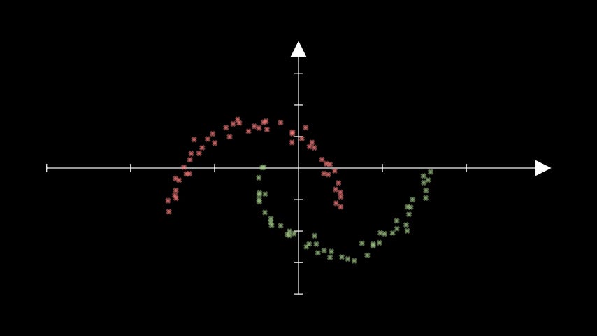
Observe what happens when we apply last week’s K-Means algorithm to this data:

Hmm… it’s clear that K-Means is struggling with this one. This is a direct consequence of the centroid-based approach.

That said, is there a way to rejig our clustering approach so that we can deal with spatial data densities of more general cluster shapes?

Before reading on, think about how you might try and cluster for the sake of grouping points based on how close they are relative to each other. Could you write an algorithm down for this?

…

Assuming you’ve had a crack at the task…

… let’s get to unpacking!

Density-based clustering

The issue with K-Means for the above example is that it does not take the spatial density of the data points into account: recall that the algorithm just groups points based on which centroid they are closest to.

Here’s the idea behind density-based clustering: we initialise the first cluster at a random data point and expand the cluster based on how close its neighbours are, halting the expansion when the other data points are too far away. Once this is done, we initialise a new cluster by selecting another random unlabelled point and repeat the process.

Given a dataset D and a tolerance ε, the neighbours of the data point x are the data points that are at most ε away from x. The corresponding subset of data is referred to as the neighbourhood of x:

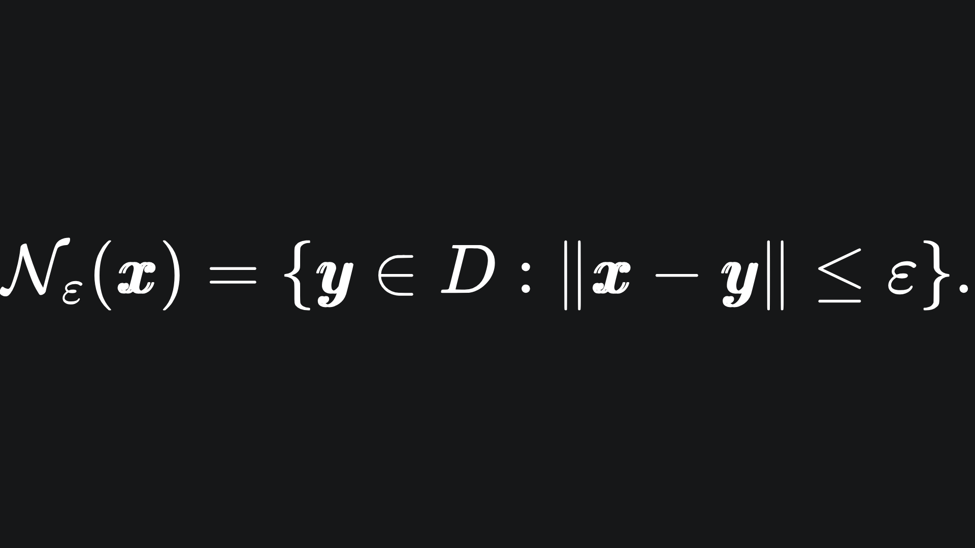
If we initialise the first cluster at x, then we will assign all the points in Nε(x) to the same cluster.

We then take each of these points and assign their neighbours to the same cluster, and repeat until there are no more neighbours at most ε away from the collection of points in the cluster. This can be dealt with in a recursive manner.²

There is one slight issue with this approach though.

Suppose that we simply expand a cluster based on any points within an ε radius. It’s likely that the cluster will swallow up the entire dataset, or at least more than we anticipated. We only want to expand the cluster at a particular point if that point has enough neighbours.

The core points in our dataset are the points that have at least minPoints neighbours, where minPoints is an integer. This allows our clusters to have borders without expanding clusters unnecessarily. The points that do not have at least minPoints neighbours are referred to as non-core points.

So by the end of the algorithm’s run, each point is either a core point, a non-core point, or an outlier. An outlier is a point that does not have enough neighbours to be considered a core point, and is not close enough to any other core point to be included in their cluster.

This gives us two parameters for the clustering model:

⚡ ε: the minimum distance a point must be away from another in order to be considered its neighbour. The smaller the value, the more restricted we are with cluster expansion.

⚡ minPoints: the minimum number of neighbours a point must have in order to be considered a core point. The smaller the value, the easier a cluster can be expanded.

Important point: in K-Means, you have to specify the number of clusters you want; however with DBSCAN, the number of clusters is determined by the parameters you pass in.

For example, if your values for ε and minPoints are too small, then most points will not have large neighbourhoods, which can force the algorithm to compensate by introducing more clusters. As such, you will most likely have to play around with the values of ε and minPoints to get a good clustering. It helps to initially plot the raw data (or at least a sample) to figure out what values would make the most sense.

The full name for this algorithm Density-Based Clustering of Applications with Noise. We shorten this to DBSCAN because, well, would you want me to write out ‘Density-Based Clustering of Applications with Noise’ every time? I thought not.

The DBSCAN algorithm

Let’s distill the arguments made in the previous section:

💥 Start the first cluster at a random core point.

💥 Scan the neighbours of this core point. For any neighbouring non-core points, simply assign them to the same cluster.

💥 For any neighbouring core points, assign them to the same cluster, scan their neighbours and repeat the process of expanding this current cluster.

💥 Once no more core points remain in this cluster neighbourhood, move on to the next cluster by choosing a random core point that has yet to be assigned and repeat the steps.

💥 The algorithm terminates when all core points have been assigned to a cluster. Any points that remain unlabelled are deemed outliers.

As for the actual coded implementation, check out my GitHub: https://github.com/AmeerAliSaleem/machine-learning-algorithms-unpacked/blob/main/dbscan.py

DBSCAN in action

Now, we apply the algorithm to data similar to what we looked at earlier. We apply the DBSCAN algorithm with ε=0.3 and minPoints=4:

Nice! The DBSCAN algorithm performs the clustering as we would expect visually.

(Sorry the animation is a bit slow, I couldn’t figure out how to make it go faster 😅)

Packing it all up

That’s two clustering algorithms in the bag! I hope the visualisations have been useful- one of the reasons I started writing this newsletter is because, back as a student, I wondered what it would’ve been like to see algorithms like clustering in an animated format. In fact, a lot of these articles are written in in the style of “what I wish I knew” when I first learnt about these topics.

Anyway, enough gushing, here’s the usual roundup:

• K-Means is suited well for spherical data clusters, but struggles with spatial densities in different arrangements.

• DBSCAN addresses this problem by clustering based on the spatial density of the data, expanding clusters based on how close the points are.

• Tuning will need to be conducted on the model’s parameters in order to get a meaningful result.

I may write a standalone article to compare clustering algorithms in greater depth. Let me know if this would be of use 👍🏼

In the meantime, I encourage you to have a play around with the code I wrote for this one. You will need the following from my GitHub repo:

dbscan.py: contains the DBSCAN implementation from scratch.

dbscan_manim.py: contains the code to animate the DBSCAN algorithm on some data from sklearn.

Training complete!

I hope you enjoyed reading as much as I enjoyed writing 😁

Do leave a comment if you’re unsure about anything, if you think I’ve made a mistake somewhere, or if you have a suggestion for what we should learn about next 😎

Until next Sunday,

Ameer

PS… like what you read? If so, feel free to subscribe so that you’re notified about future newsletter releases:

Sources

• “A Density-Based Algorithm for Discovering Clusters in Large Spatial Databases with Noise”, by M. Ester, HP. Kriegel, J. Sander and X. Xu: https://dl.acm.org/doi/10.5555/3001460.3001507

• The following resource helped me write my dbscan.py file: https://github.com/xbeat/Machine-Learning/blob/main/Building%20DBSCAN%20Clustering%20Algorithm%20from%20Scratch%20in%20Python.md

• My GitHub repo where you can find the code for the entire newsletter series: https://github.com/AmeerAliSaleem/machine-learning-algorithms-unpacked

1. This data came from one of sklearn’s pre-prepped datasets: https://scikit-learn.org/stable/modules/generated/sklearn.datasets.make_moons.html

2. Recursion is something we mentioned briefly in the decision tree article from a few weeks ago: