
Decision tree deep-dive: information gain and Gini impurity
Explaining the decision tree's greedy recursive nature and the maths behind splitting criteria, with images and animations to depict the steps.

Hello fellow machine learners,
Another week, another MLAU article! We spent last week discussing how to measure information, and will be using some of that knowledge now to help us understand a simple yet surprisingly powerful classification algorithm: the decision tree.
No more waffling, it’s time to unpack!
Binary splits
Our setting is once again a dataset where each row is attributed a discrete label. For the visualisations in these articles, I usually represent the labels of data points by the colour of the data point, usually either red or green. But don’t forget real-world contexts: for example, our dataset could describe the information of medical patients, where the label tells us whether each patient has a specific illness or not.
When we discussed the Support Vector Machine a few weeks ago, we explained how it uses a ‘separating hyperplane’ approach to split data points with one of two labels. The SVM had some methods for dealing with linearly inseparable data, but those methods relied on somewhat complicated maths.
Take the setup depicted in the below image for example:
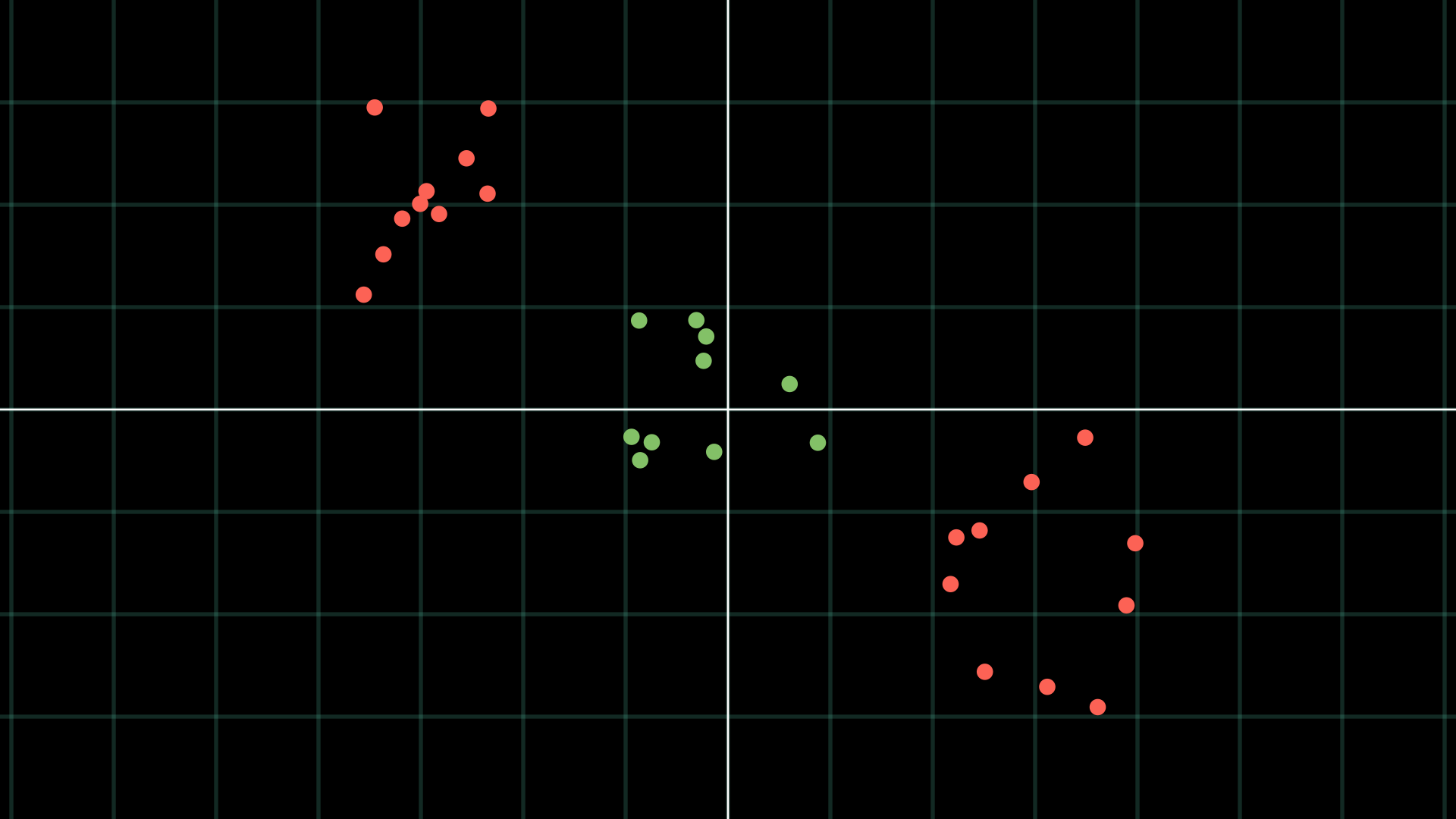
The SVM would struggle to classify this data without using a feature map.
But here’s an idea: instead of using the SVM’s higher-dimensional feature maps/slack variables, why not just stay in the same feature space, but separate our data using a combination of linear decision boundaries? Here is what I mean:
In the above, we first classify any points (x,y) with y>1 as red. This leaves us with the points below the line y=1. For these remaining points, we colour the points on the left of the line x=1.5 green, and those on the right side red.
The main point here is that we are able to create a non-linear decision boundary by combining two linear decision boundaries together! Pretty cool, right?
Simplicity is key here:
For each of these boundaries, our split will only concern an individual feature of the dataset. This means that each individual decision boundary will be parallel to one of the axes of the space we’re working in. So in 2D, our splits will be parallel to either the x-axis or the y-axis.
Each split will be binary, i.e. the data will be split into two regions by each individual decision boundary.
How do we conduct the ‘best’ splits?
What does it even mean for an individual split to be the ‘best’ one anyway?
Well, let’s think about the criteria we wish to satisfy:
We want each resultant region from our splitting process to be homogeneous, i.e. all the data points in each region should belong to the same class. In ML, we sometimes remark this as purity in each resultant region. In our visual context, we ask that each region consists of only red points or only green points, but not both.
We want to get to these groups with as few splits made as possible. This means that each each split we conduct must be sufficiently meaningful.
Every split produces a pair of regions, on which we can conduct further splits. Hence, the method we are describing is recursive in nature. So regarding the first condition, we apply a split, and then apply another split in each subsequent region. We continue this process until we achieve data purity in each region.
This technique is called a ‘divide-and-conquer’ approach.
To satisfy the second condition, we want to gain as much information as possible from each split. We can relate this to information entropy: we want to minimise the entropy associated with each split we conduct, and continue to split until each resultant group is pure.
With all this in mind, we have essentially described how a decision tree works: the resultant classification regions correspond to the leaves of the tree; and the binary splits refer to the tree’s branches.
The decision tree corresponding to the previous animation is shown below. Note that I have used x_1 and x_2 for the axes here instead of x and y. This is because we usually use ‘y’ for the labels when it comes to supervised learning problems:
Important note here: the splits conducted are considered the ‘best’ only within the local scope of samples. The tree is not looking multiple splits into the future or anything like that, so the approach is somewhat myopic. Just something worth bearing in mind as we get into the next section.
Splitting criteria
The decision tree algorithm comes equipped with a few methods of measuring how good a split is, with the aim of making all the leaf nodes pure. Recall the information entropy formula from last week: the entropy of a probability distribution P = (p_1,…,p_n) is given by
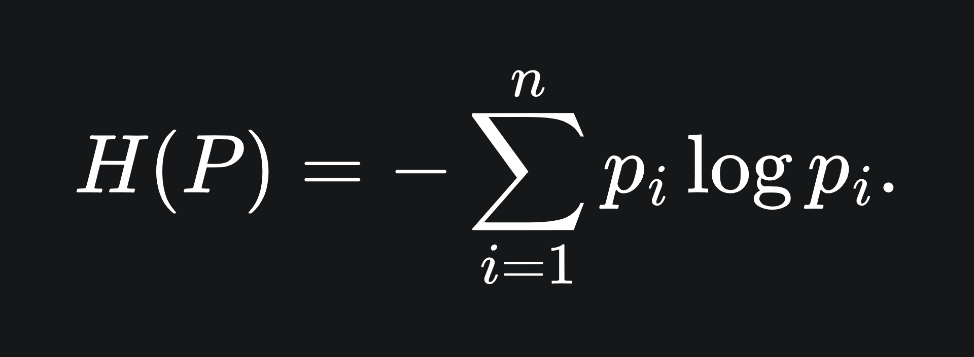
We want to group the data points into pure leaf nodes. This means we want a low amount of surprise from the data labels in each leaf, which corresponds to minimising the entropy of each leaf. So the lower the associated entropy, the more homogeneous each classification region is, which is ideal.
The decision tree comes with a few built-in methods of determining the best splits to conduct. These are called splitting criteria. The two main ones used in scikit-learn’s decision tree implementation are information gain and Gini gain.
Information gain
Information Gain: it does what it says on the tin, although the formulas might look a bit funky. This splitting rule provides a measure for how much information is gained from a split. The Information Gain obtained from splitting a set of data S on the feature A is given by

where H(S|A) is the conditional entropy incurred from splitting on the feature A:
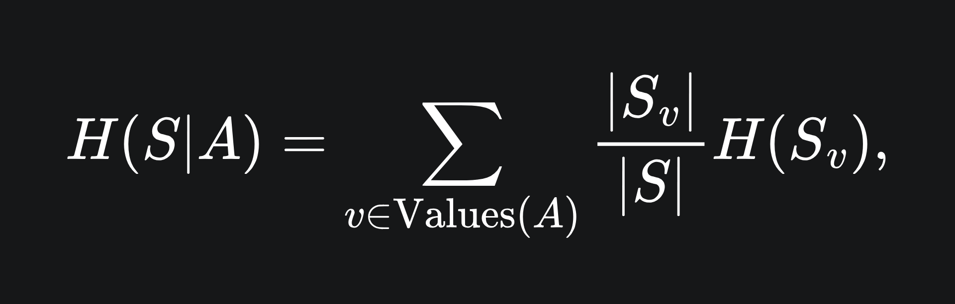
where S_v is the subset of the dataset S for which the rows have label v:
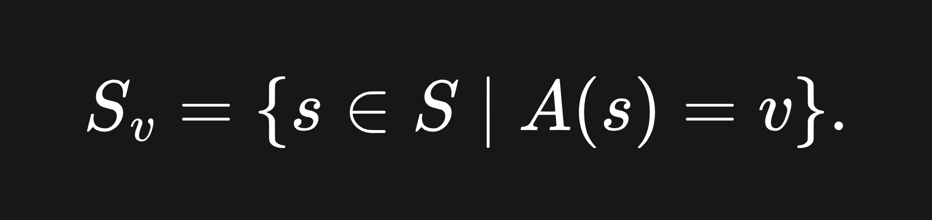
This all looks like a lot of mathematical slop, but the idea is to take each possible value in the column A and sum up all the corresponding weighted entropies.
We then subtract these weighted entropies of the potential splits on attribute A from the entropy of the current dataset in consideration. If the weighted entropies are large, then the information gained from splitting on attribute A will be small.
Gini impurity
The Gini impurity provides an alternate set of criteria we can use to split our data.
Suppose that, under a proposed data split, the classes of data in one of the resultant nodes are {1,2,…,n} which each arise with empirical probabilities p_1,…,p_n respectively.
The Gini impurity of a particular node measures the probability that a data point is labelled incorrectly in this node:
In the above: the fourth line uses the fact that events in question are disjoint; and the sixth line uses the independence of the events.
Gini gain
The information gain formula uses entropy. But if we use the Gini impurity formula instead of entropy, the result is called the Gini gain:

The main difference between the two methods is the computational complexity involved. Logarithmic functions are more resource-intensive to compute, and so Gini gain may be faster to compute in reality.
What could go wrong?
So the decision tree can take a labelled dataset and classify the data points by conducting the splits that best work to separate the data into pure leaf nodes.
That sounds great! Perfect, even! What could go wrong?
I’ll leave you to have a think about it for now- we’ll do a full breakdown next week.
Packing it all up
This article has demonstrated how information entropy can be applied for the sake of supervised classification. We’ve got plenty more to discuss regarding tree-based algorithms, but for now, here is a summary of today’s discussion:
A non-linear decision boundary can be decomposed into a combination of linear decision boundaries.
The decision tree algorithm aims to conduct data splits so as to yield leaf nodes of the highest purity (i.e. all nodes in each leaf hopefully belonging to the same class).
The information gain and Gini gain are two examples of splitting criteria that can help us figure out what the ‘best’ splits are.
Training complete!
I hope you enjoyed reading as much as I enjoyed writing 😁
Do leave a comment if you’re unsure about anything, if you think I’ve made a mistake somewhere, or if you have a suggestion for what we should learn about next 😎
Until next Sunday,
Ameer
PS… like what you read? If so, feel free to subscribe so that you’re notified about future newsletter releases:
Sources
“The Elements of Statistical Learning”, by Trevor Hastie, Robert Tibshirani, Jerome Friedman: https://link.springer.com/book/10.1007/978-0-387-84858-7
Decision tree classifier documentation from scikit-learn: https://scikit-learn.org/stable/modules/generated/sklearn.tree.DecisionTreeClassifier.html