What is the cross-entropy loss for an ML classifier?

How to measure model performance with loss functions.

Hello fellow machine learners,

I am officially back in the UK, although I certainly haven’t missed the humidity that comes with British summer 😓 I much prefer the breeze from the stands in the Hungaroring…

Anyway, I wrote an article a few months ago about performance metrics for classification models. In case you missed it, I have linked it below. Trust me, it’s a certified banger:

Performance metrics are used to evaluate how well a model has done at its classification task after training. But there are some ML models that need to know how well they’re performing during training, in particular with respect to the model parameters, so that they can adjust their future training iterations.

This is where the loss functions come into play. A loss functions aims to quantify how badly a model has done in making its predictions.

Read on to find out more about different types of loss function for classification tasks!

What is a loss function?

A loss function attaches a numerical value to the predictions made by a model. The larger the loss, the less good the predictions are. Our aim is to minimise the loss for a given set of input data.

Let’s begin the simple case of binary classification: given a dataset of n points

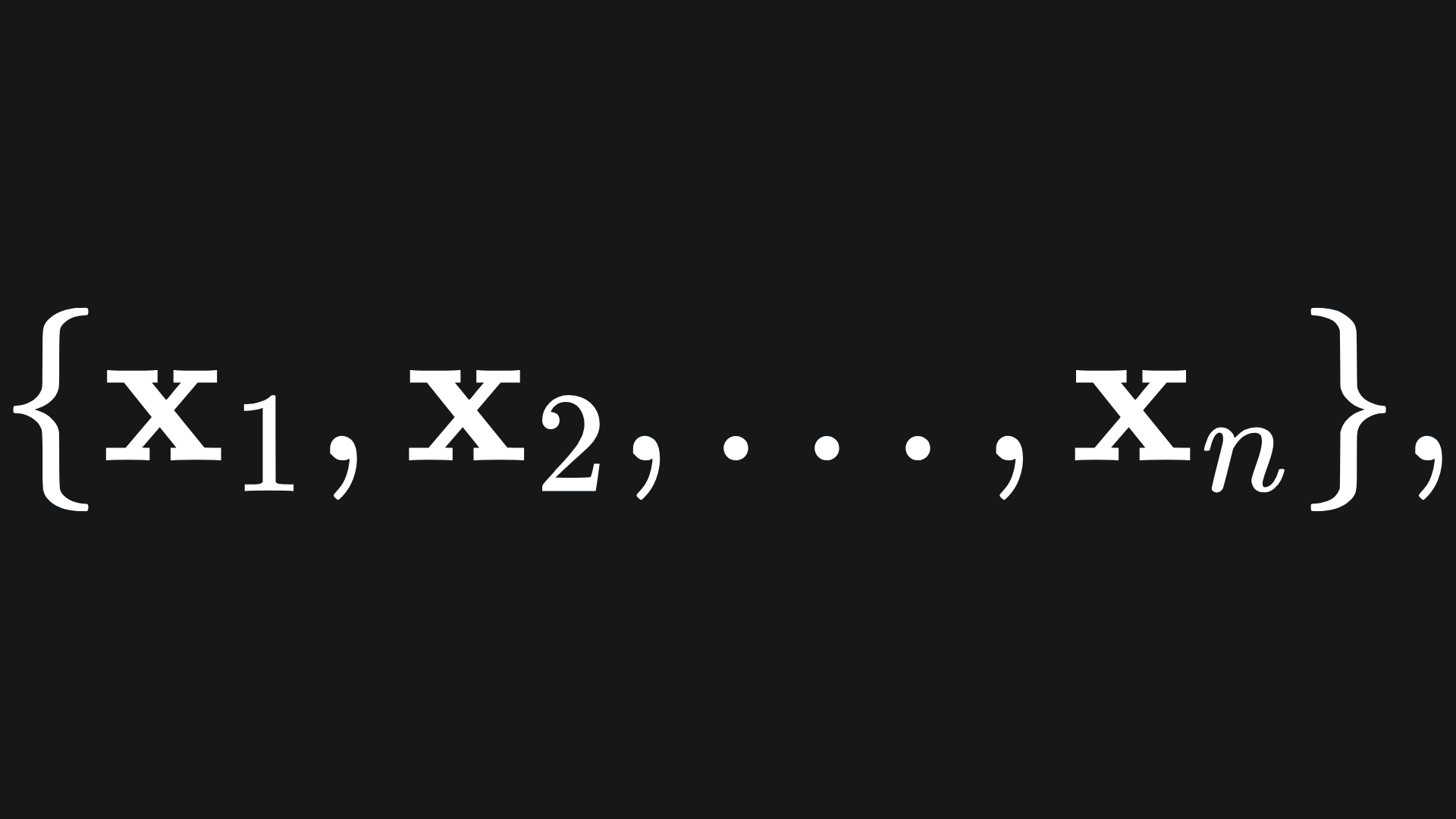
where each point is assigned a label

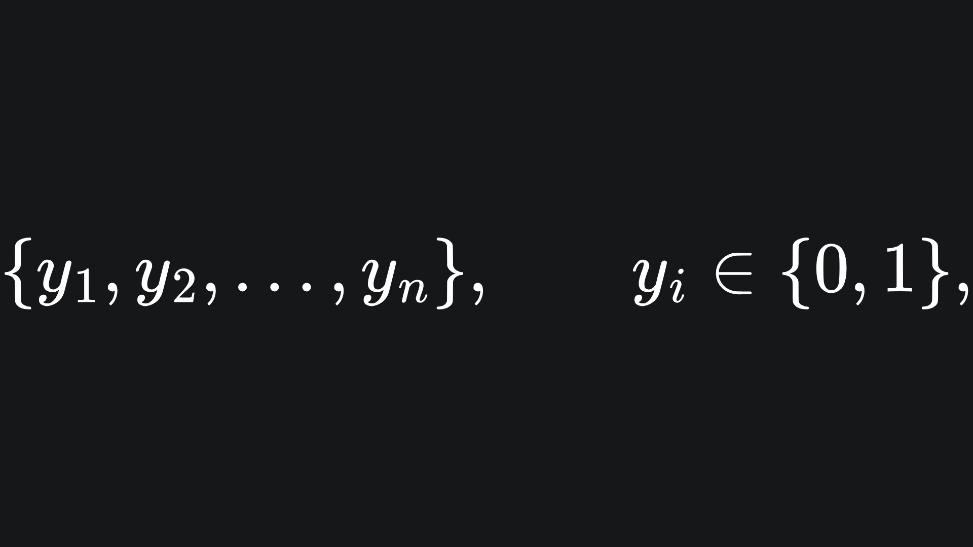
the classifier is tasked with making predictions

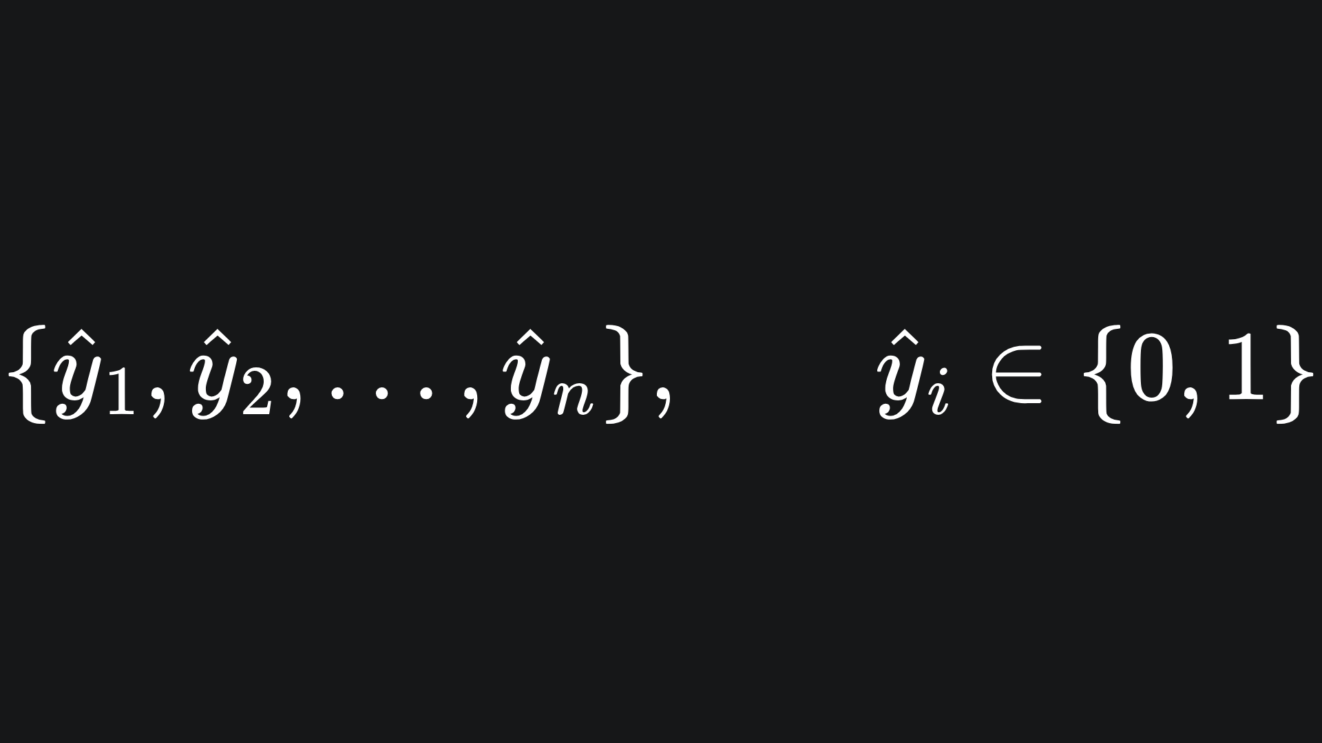
that resemble the true labels as closely as possible. We will encode the true labels together in the vector y, and similar for the predicted labels with ŷ.

0-1 loss (aka Indicator loss)

The simplest loss function we could cook up is the one that literally counts the number of mismatches between the predicted labels and true labels, then normalises the result:

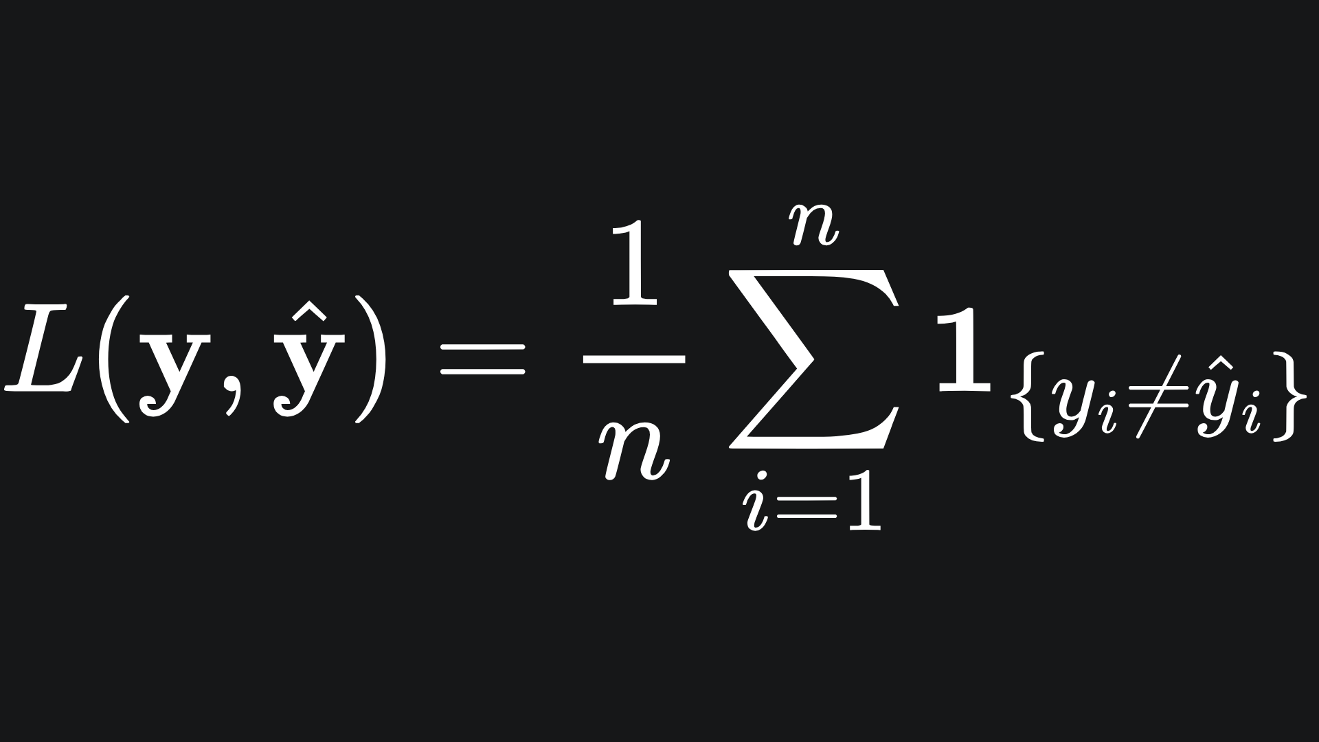
You can think of this as the fraction of misclassified samples. Recall the indicator function defined as

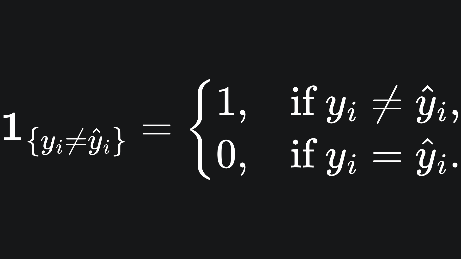
So if the prediction vector matches the true vector perfectly, we get a loss of 0. But if the prediction vector gets every prediction wrong, we incur a loss value of 1.

The construction of this loss function is nice and intuitive, since it’s essentially just an exercise in counting. However, it is not differentiable¹: this is a useful quality that we will explore the value of in a future article.

In fact, the 0-1 loss function is not even continuous², since it can only take the values between 0 and 1 that are multiples of 1/n.

Binary cross-entropy (aka Log loss)

Our next aim is to construct a continuous, and hopefully smooth, loss function that preserves the idea that the loss is large for significant misclassification, yet small for a sequence of good predictions.

A lot of the classification models you’ll interact with operate under a probabilistic system. Take the logistic regression model as an example: the output of this model is a float value between 0 and 1. The larger the value, the more ‘confident’ the model is in the prediction of the label {1} for that particular data point.

We can use these probabilistic outputs to construct the binary cross-entropy loss function, the formula for which is

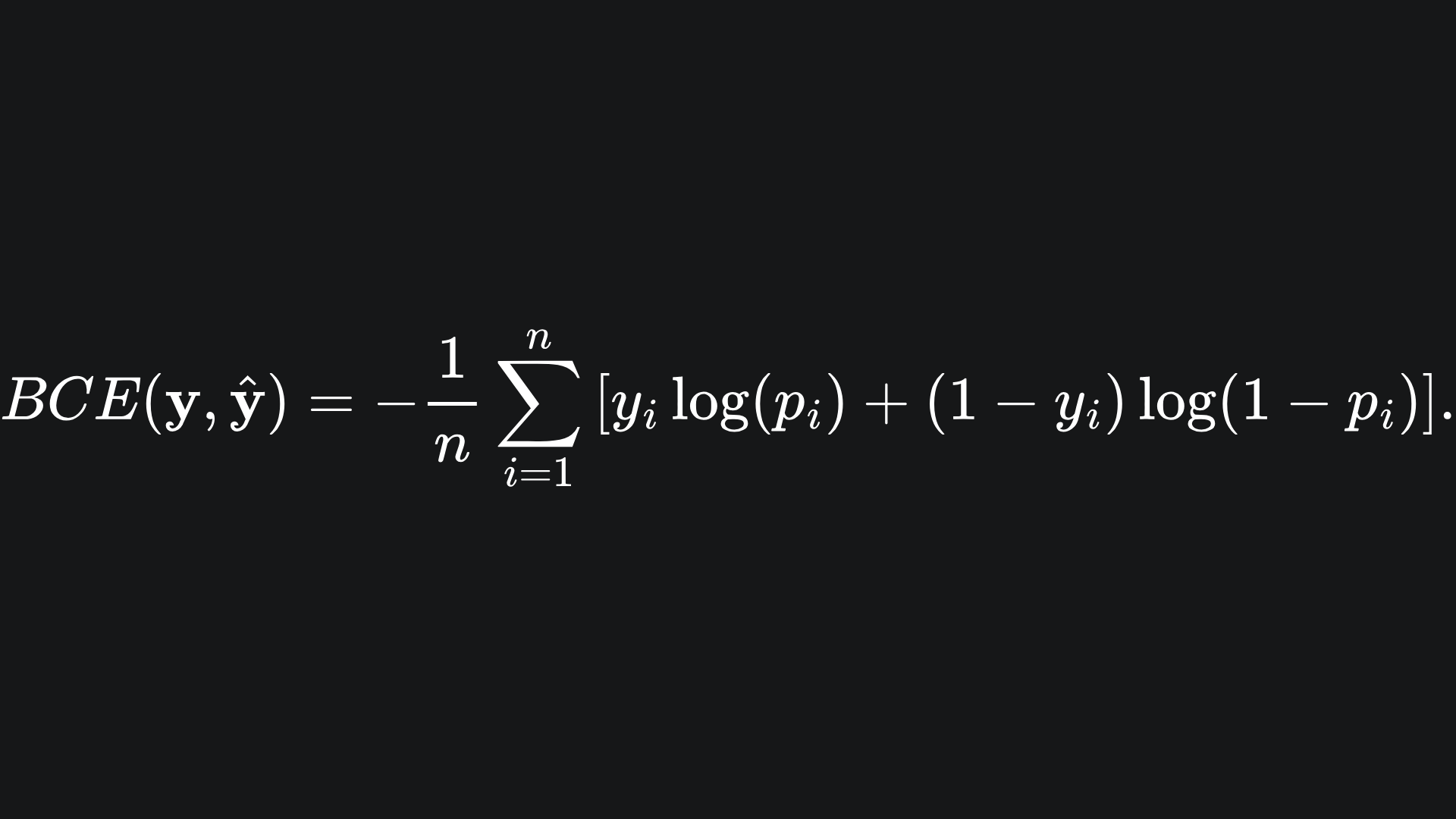
Here is what it looks like. (Source: MLAU GitHub)

Remember: we’re assuming that the true labels are either 0 or 1. So in the plot, all we really care about is the behaviour of the surface at those two values for all possible values of p. In particular, the loss spikes at the major mismatch areas between the predicted and actual labels:

💡 If y_i=1, then the summand of BCE becomes

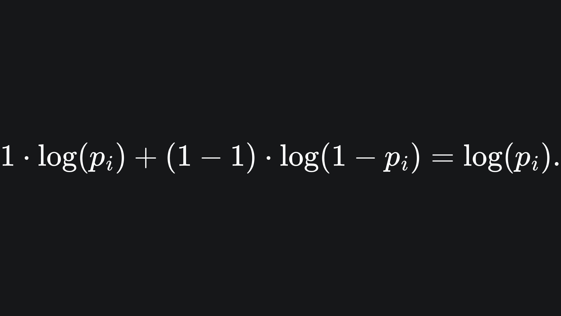
The logarithm takes large negative values for inputs in the range (0,1), but don’t forget the negative prefactor in front of the summation! This leaves us with a large positive loss for probabilities that are not equal to 1, and zero loss for that particular data point otherwise. So the closer the match of p_I to y_i, the smaller (and hence better) the loss.

💡 If y_i=0, then the summand becomes

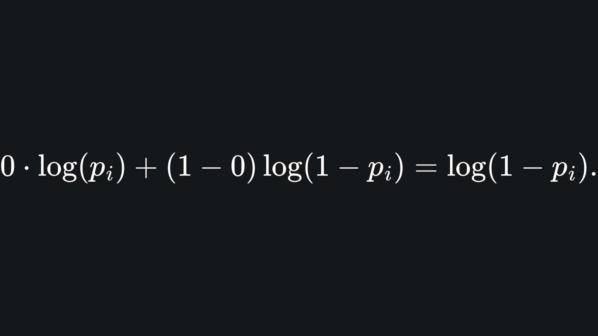
We can argue similarly as in the first case- we want the value of p_i to be as close to 0 as possible since the minimum possible loss is achieved at log(1-0) = 0.

A mathematician’s pendaticness

What happens at p_i=0? Technically speaking, log(0) is undefined. Mathematically, we say that

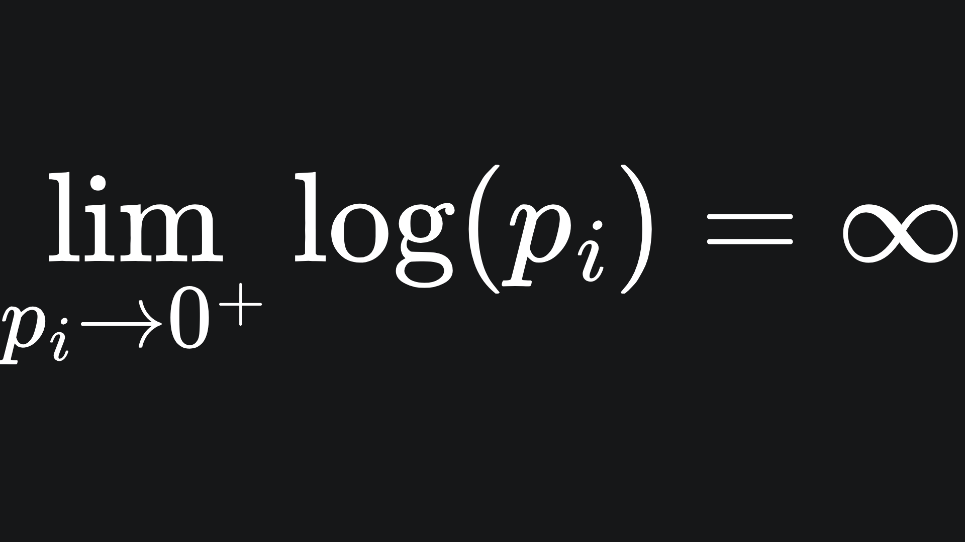
Computationally, we usually just take the value of p_i to be close to 0 rather than actually zero, which helps us circumvent the issue of “infinite loss”.

So if y_i=1, then we get a very large loss value, which makes sense for a loss function. And if y_i=0, then we just multiply this log value by 0 and get zero loss anyway.

Similar logic applies for when p_i is close to 1 for the other logarithm term.

Categorical cross-entropy

The BCE loss from the previous section can be extended to deal with multi-class classification problems. For instance, if the true labels y₁,…,y_n could take any value from the set {1,2,…,m} for m>2, then we are no longer in the binary classification setting from before. A real-life context for this could be e.g. an NLP task where you’re trying to classify sentences as being either positive, negative or neutral in sentiment (m=3 here).

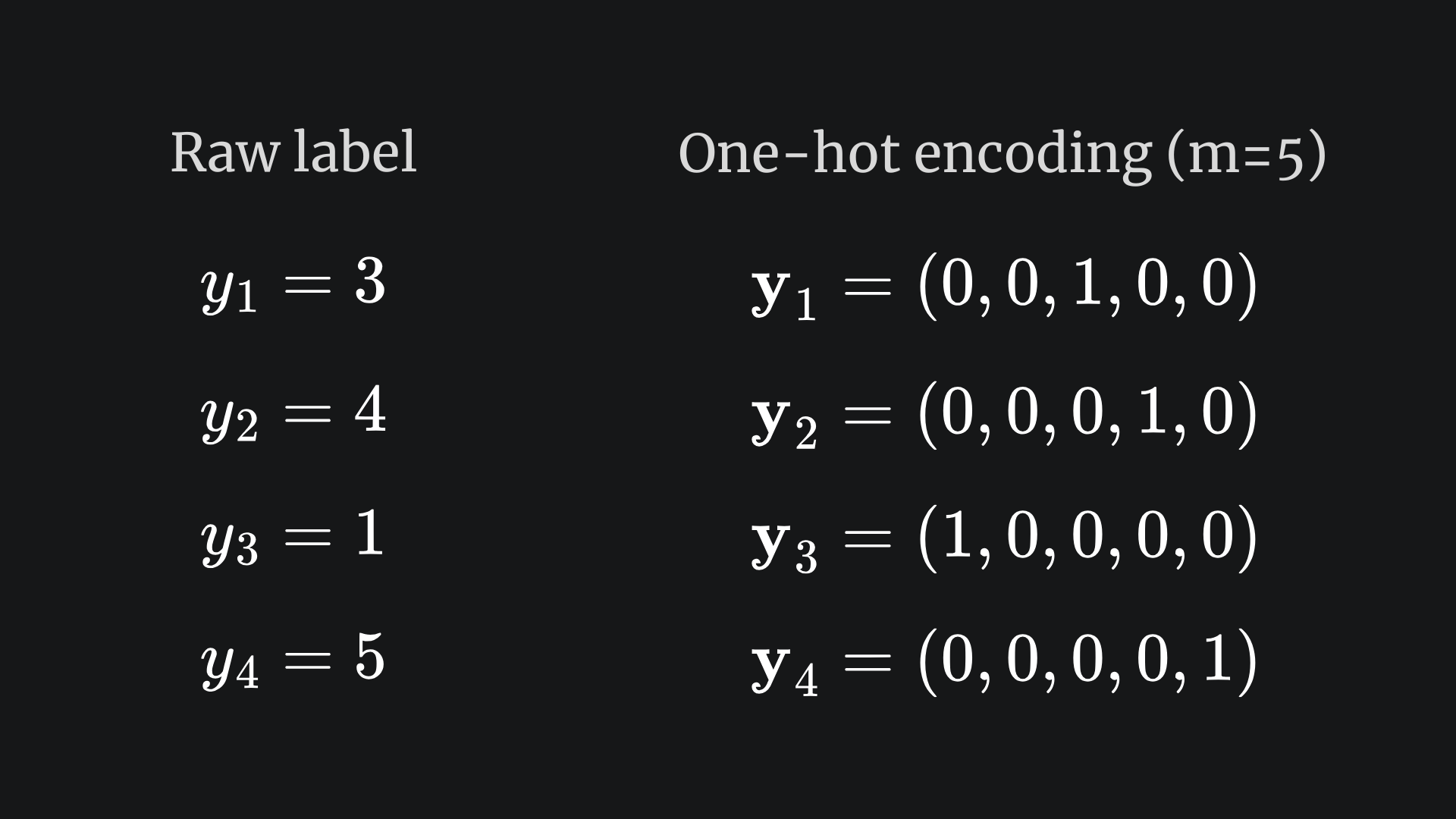
How can we deal with this? The first thing we do is one-hot encode the labels y₁,…,y_n. Essentially, we take each one and make it an m-dimensional vector with the value 1 at the y_i-th position and the value 0 elsewhere. Here is what that looks like:

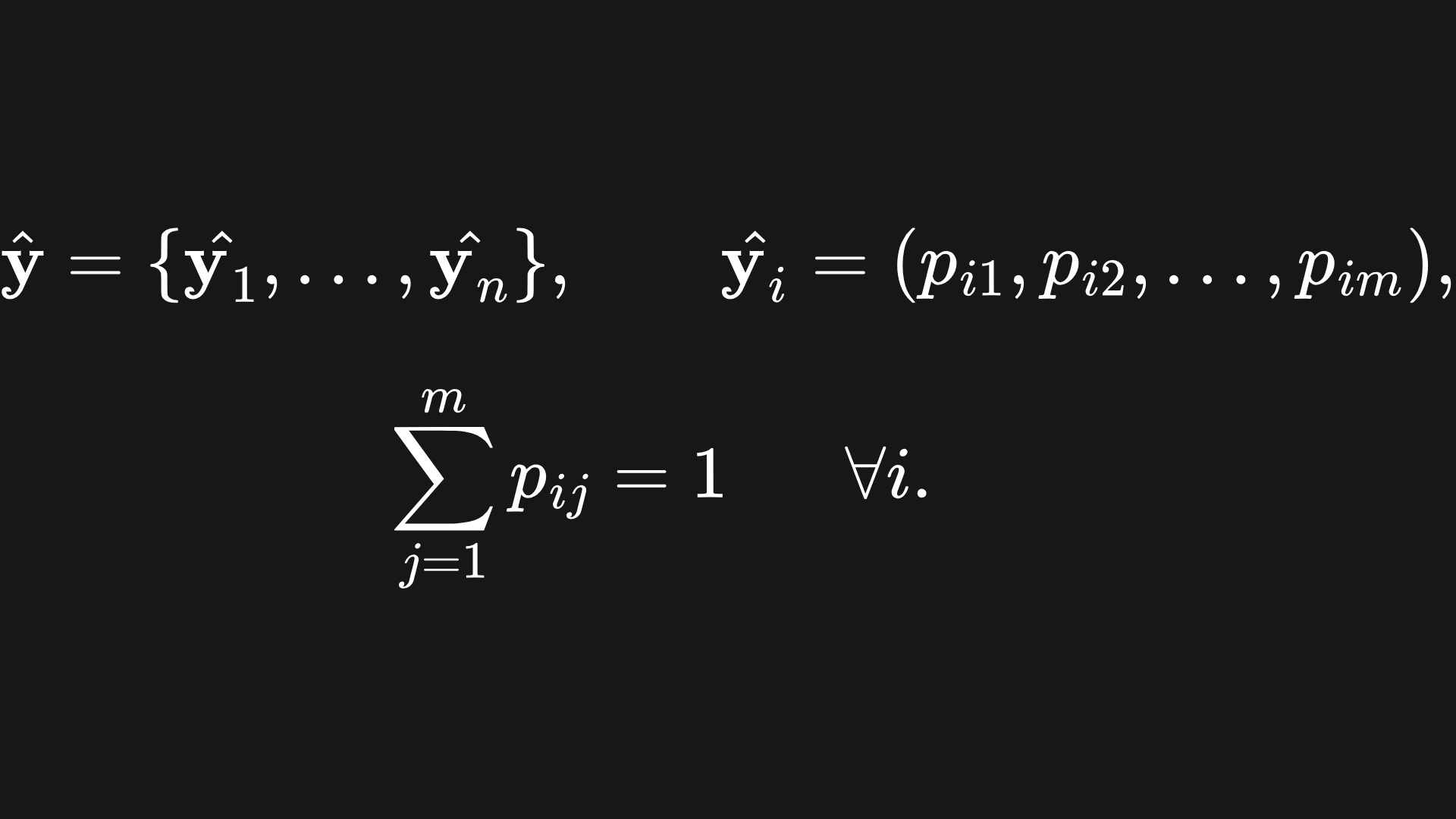
For multi-class problems, the predicted labels are in fact vectors. The elements of each vector sum to 1:

Now, we’re in a position to define the categorical cross-entropy: by extending the BCE formula across the m classes:

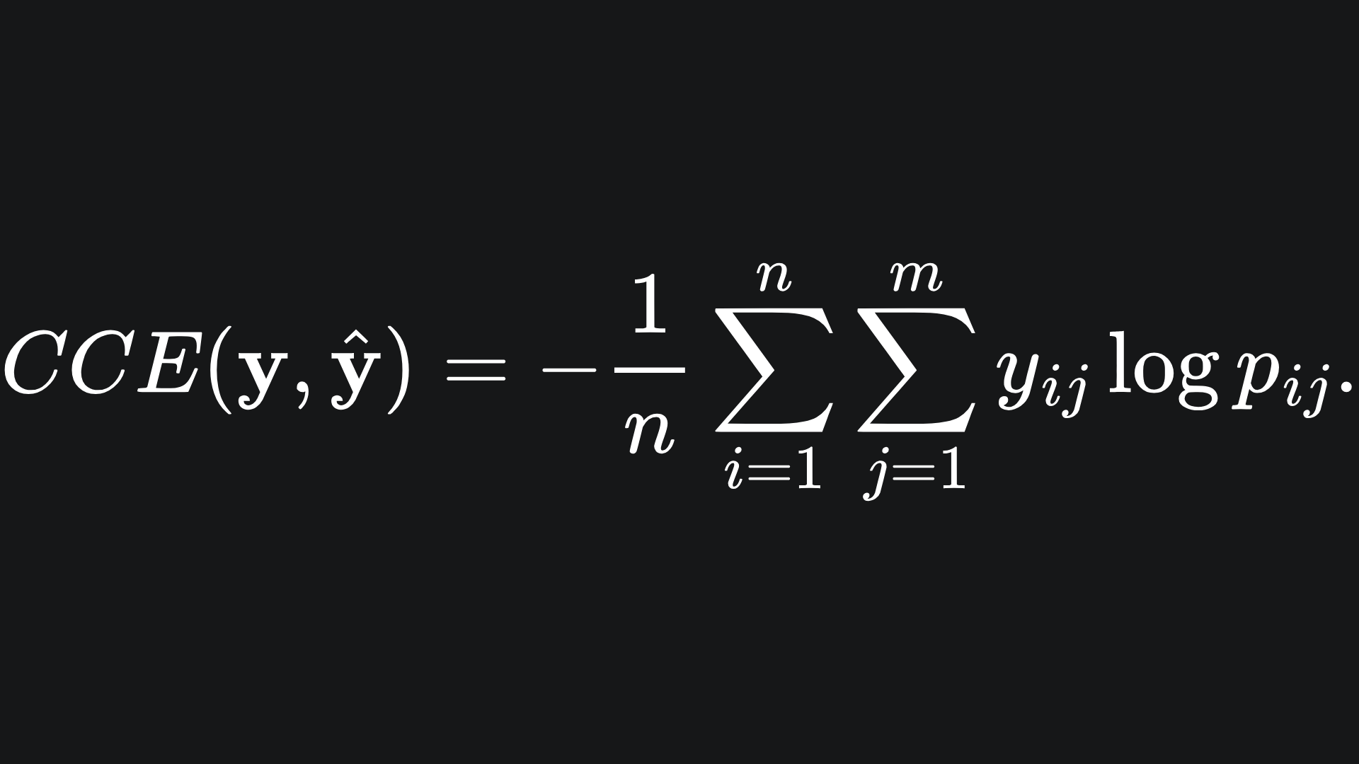
For the i-th data point, we multiply together the predicted label values with the corresponding log probability prediction values. As with BCE, strong matches with incur smaller losses.

Packing it all up

The utility of loss functions will be made evident down the line. For now, we’ve cooked up a way of quantifying the ‘incorrectness’ of predicted classification labels. Crucially, these functions are expressed with respect to the predictions themselves.

Now for the usual roundup:

❓ The 0-1 loss simply counts the number of prediction mismatches and normalises the result. This formulation is intuitive, but the loss function is neither differentiable nor continuous (boo!).

❓ Binary cross-entropy fixes the problems of 0-1 by smoothening out with the logarithm function. The intuition of “good predictions, less loss” is also preserved.

❓ Categorical cross-entropy is an extension of binary cross-entropy to more than 2 classes. It works by one-hot encoding the true labels and multiplying these with the log of the predicted probability vector values.

Training complete!

I hope you enjoyed reading as much as I enjoyed writing 😁

Do leave a comment if you’re unsure about anything, if you think I’ve made a mistake somewhere, or if you have a suggestion for what we should learn about next 😎

Until next Sunday,

Ameer

PS… like what you read? If so, feel free to subscribe so that you’re notified about future newsletter releases:

Sources

• My GitHub repo where you can find the code for the entire newsletter series: https://github.com/AmeerAliSaleem/machine-learning-algorithms-unpacked

1. For now, you can think of a differentiable function as a function that is smooth. The mathematical definition of differentiability is a lot more involved than this, but we won’t worry about that for now.

2. For now, you can think of a continuous function as a function that can be drawn on a sheet of paper without you having to lift your pen off the page. Again, this is a big simplification!