
Choosing the right performance metrics for classification models
Understanding, accuracy, precision, recall, etc. using the confusion matrix, and describing example use cases for each.

Hello fellow machine learners,
I would like you to picture yourself in the following scenario:
You have been tasked with building a machine learning model to help detect whether medical patients have contracted a rare disease. This disease is so rare that the probability of a patient being infected with it is 1%. Your superiors want you to build a model which attains the highest accuracy. This will be a binary classifier which takes a patient’s information as input, and then tells you whether the patient has the disease or not, which we could encode in the output as either 1 or 0 respectively.
Flexing your ML skills, you spend the next few working days building a model which attains an accuracy score of 85%. Nice work!
Yet your joy is short-lived, as your superiors inform you that a far simpler model has been built by another member of the team in about 10 minutes, which achieves 99% accuracy with ease.
Huh??!! What’s going on here? Is the other team member a super genius, has your company given bad instructions, or are you not as good an ML practitioner as you thought?
Read on to not only find out, but to also understand the following animation:
Let’s get to unpacking!
Performance metrics
As with anything in machine learning, we should always start from first principles and definitions.
We begin with the confusion matrix, which illustrates how well or poorly our model makes predictions. For our binary classification problem, this will look like a 2x2 grid: the first column gives the number of patients that actually have the disease, the second column gives the number of patients that do not have the disease; and the rows correspond to the predictions made by our model. Here is an example:
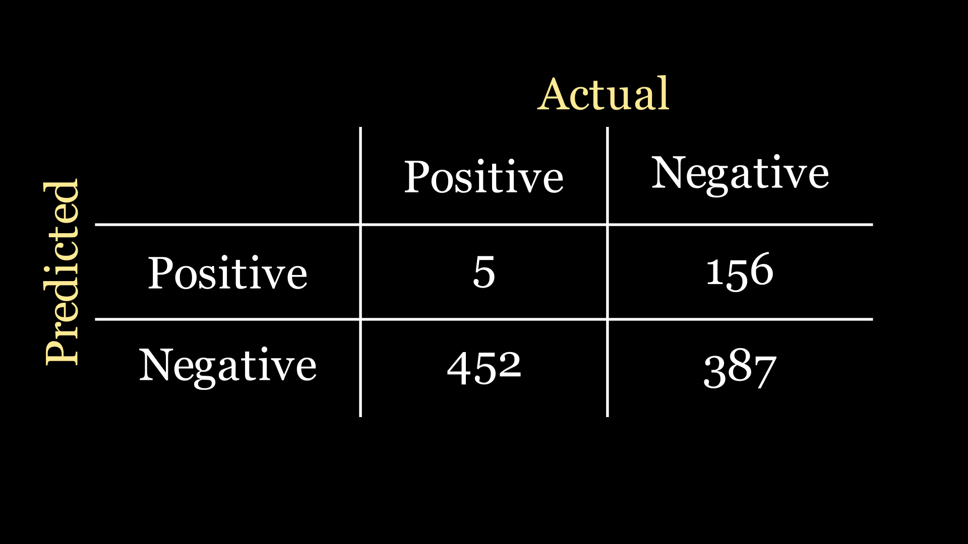
From now on, we will call a detection of the disease a ‘positive’ result, and absence of disease detection a ‘negative’ result. That is to say, we receive a positive signal from the model when it thinks it has detected an instance of the disease.
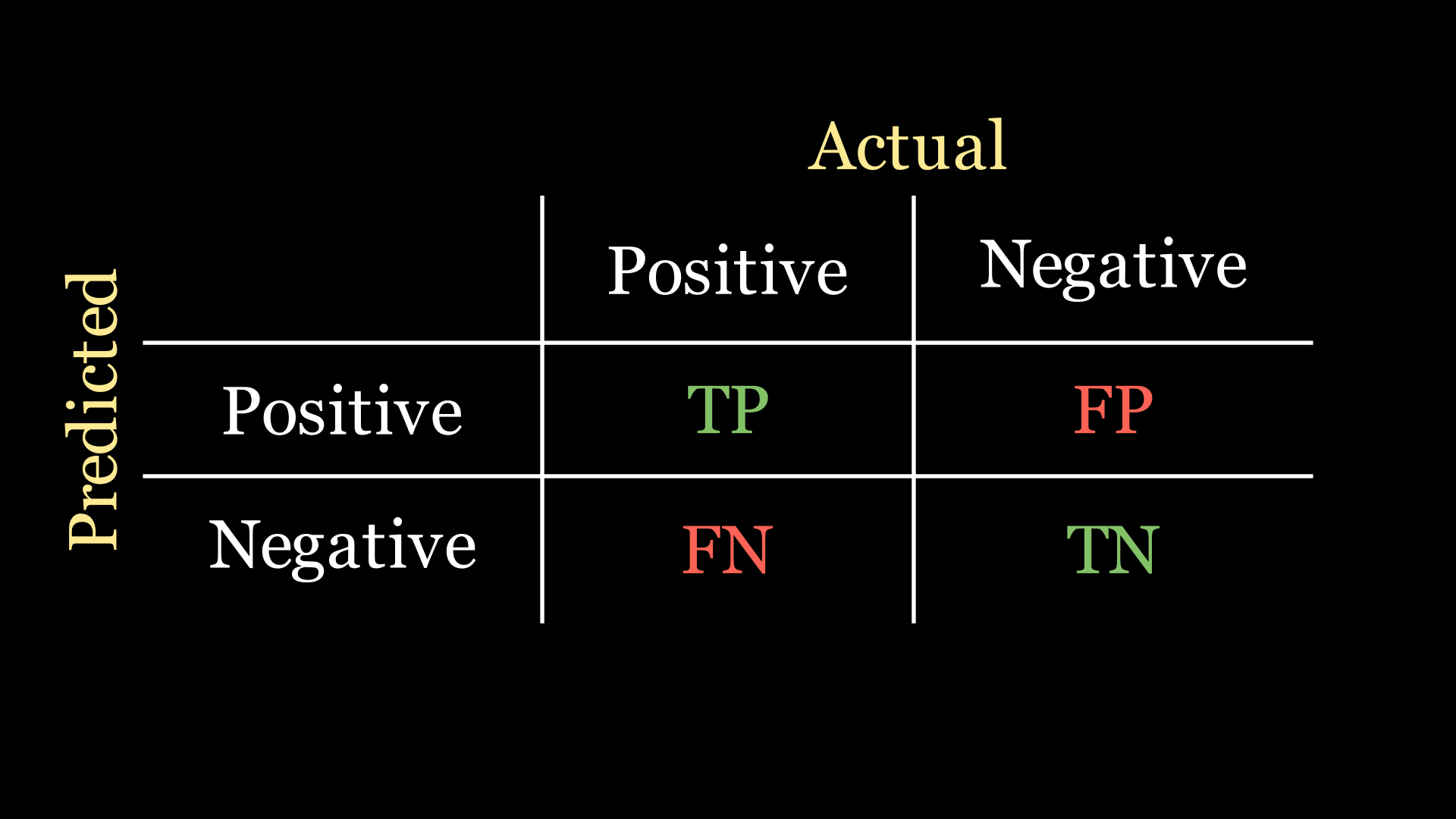
Each cell in the confusion matrix represents a certain quantity:
True positive (TP): the the number of patients the model predicts to have the disease, who actually have the disease.
False positive (FP): the number of patients that the model predicts to have the disease, who actually do not have the disease.
False negative (FN): the number of patients that the model predicts as not having the disease, who actually have the disease.
True negative (TN): the number of patients that the model predicts as not having the disease, who actually do not have the disease.
Here is a depiction of what this looks like on the confusion matrix:
Recall that your company wanted you to build a model to optimise accuracy. The accuracy of a classifier is the proportion of points that are correctly classified:
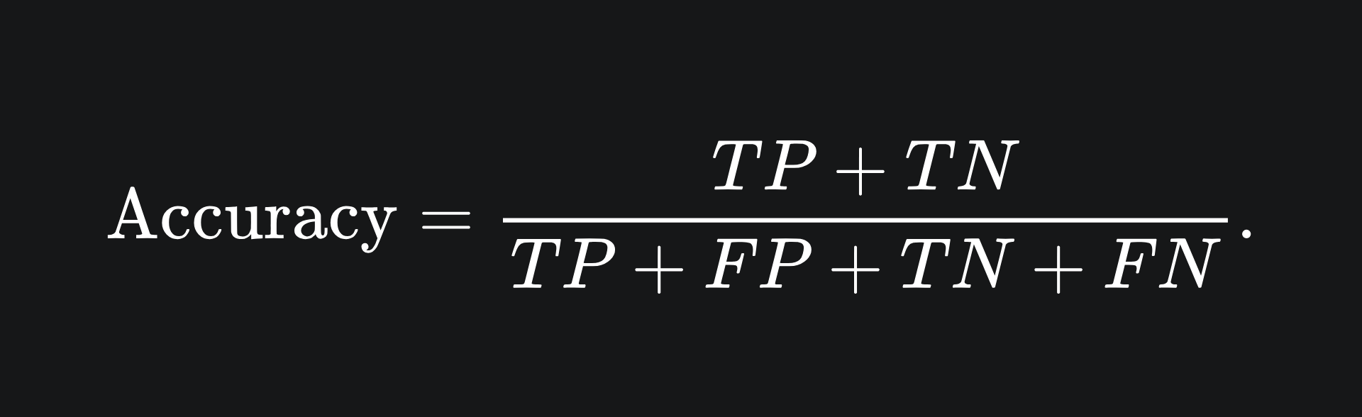
Since this is a proportion, the accuracy value will be between 0 and 1, and we can convert this into a percentage if we wanted.
Medical marvel
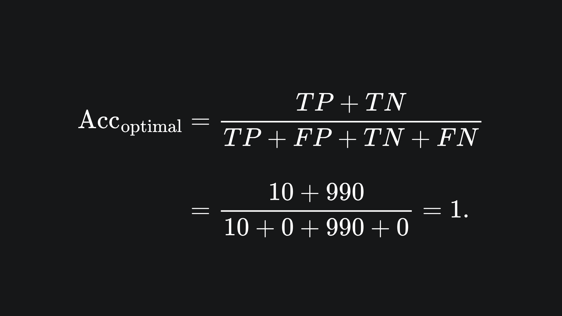
Let’s pause and have a think about the classification task that our company gave us. We know that only 1% of the patients in our data actually have the disease. So if we had n=1000 patients in our dataset, only 10 of them actually have the disease. The best confusion matrix scenario for a classifier for this problem would be the following:
In fact for any confusion matrix, the most optimal classifier is the one whose confusion matrix only has values along the main diagonal.
The accuracy for this classifier, following the formula outlined above, is
❓ Can you see how we could build a super simple classifier that achieves an accuracy of 99%?
…
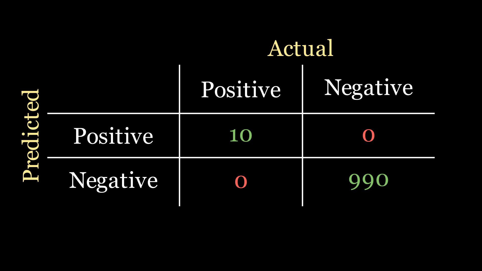
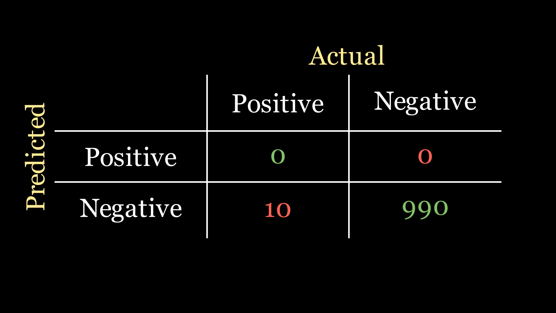
💡 We can just predict every patient as not having the disease. Is is called a naive classifier, the confusion matrix of which looks like:
and the corresponding accuracy score is now
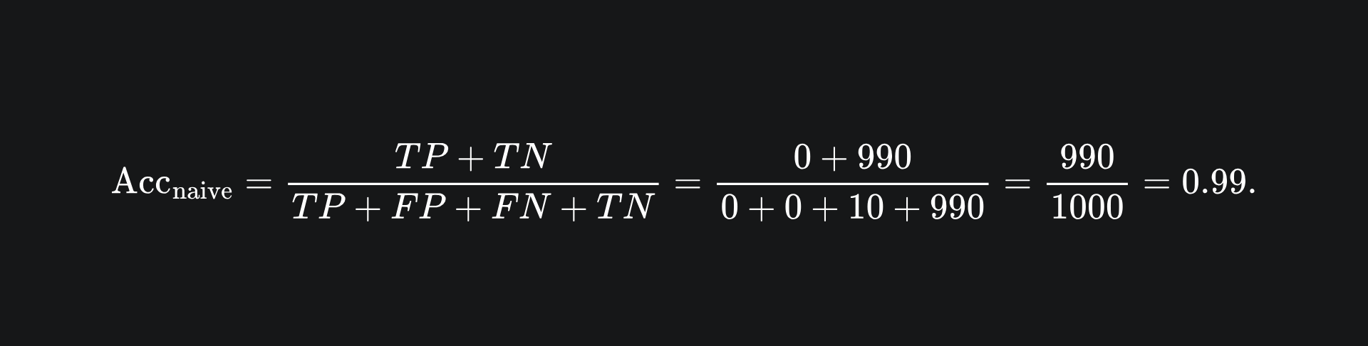
Ta-da! 99% accuracy achieved with barely any work. Now we know how our colleague achieved such a high accuracy with such ease…
But the more important question is whether or not our colleague’s classifier is a good one. Despite the high accuracy, by the way it’s designed it doesn’t actually detect any instances of the disease at all! It just defaults to saying that no disease is present for any data instance.
Here is the main issue: the accuracy metric is not suited to datasets of major class imbalance, such as the example one we’re discussing.
So it’s not always a good idea to use accuracy as the performance metric of our models. What do we do instead then?
Recall
Given the context of disease diagnosis, we want a classifier that prioritises the detection of the disease in question. A metric we can use for this is recall:
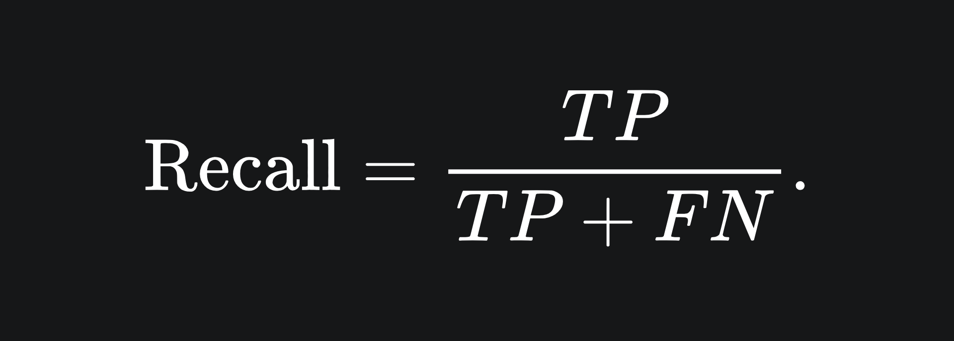
The recall of a classifier tells us the proportion of patients that were classified as having the disease, that actually have the disease.
Another of way of saying it: out of all the patients the model predicted as having the disease, what percentage actually have it?
This metric is better than accuracy for our use case because, for the sake of medical diagnosis, we do not want our model to miss any instances of the disease. We’re not too concerned with how many false positives the model outputs (i.e. model predicts infection when the patient doesn’t actually have the disease). Rather, we need to keep the false negative value as low as possible, otherwise we’ll have patients who have the rare disease but may not know it.
Although false positives are inconvenient, false negatives are detrimental.
Let’s see what the recall of the naive classifier looks like:
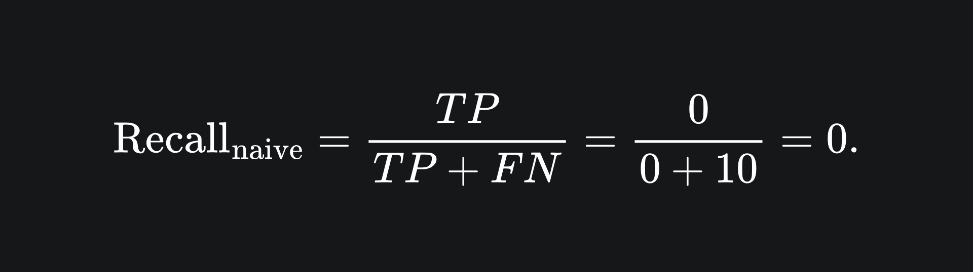
Ah, now that’s more like it.
Precision
The recall performance metric is important in cases where we do not want too many false negatives. But what about contexts where the flagging of false positives is too inconvenient to ignore?
Precision is another performance metric, which measures the proportion of positive classifications that were actually positive:
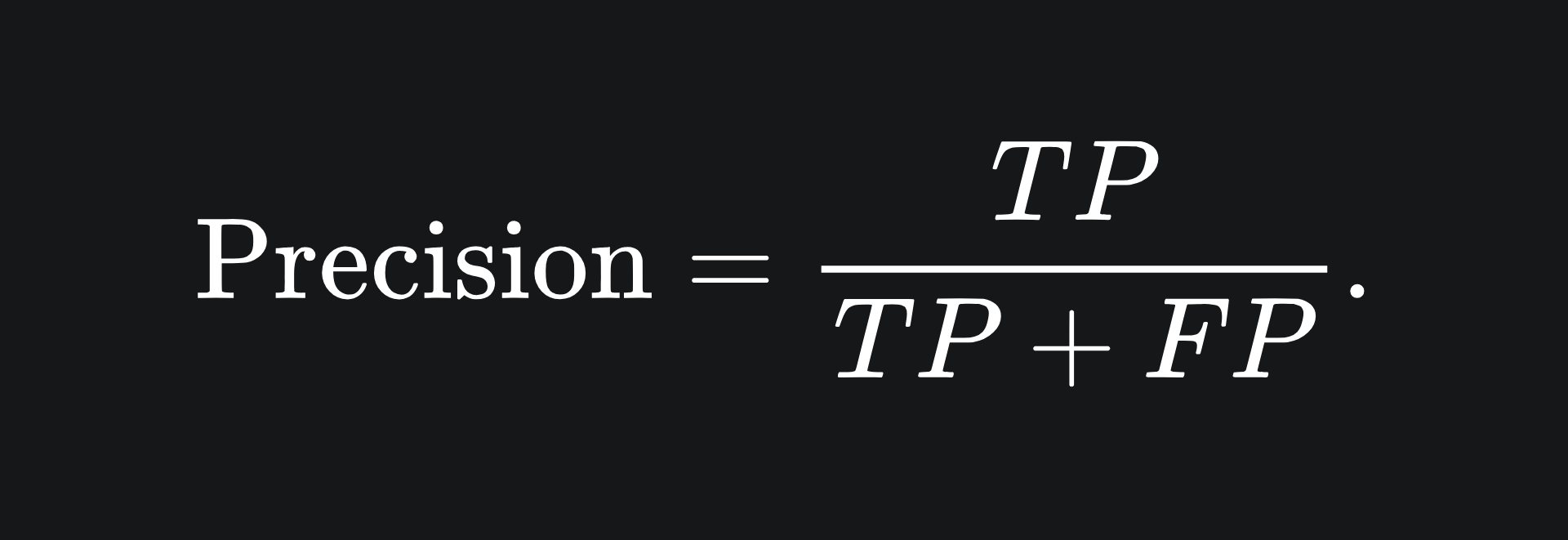
This metric is useful when you want to emphasise to the model that you don’t want false positives unnecessarily flagged. This could be useful in the context of, for example, email spam detection; a surplus of false positives may mean that important emails may end up in your spam folder! This would certainly be unideal.
F1 score
Your problem context may require some combination of flavours from both precision and recall. The F1 score provides a balance between precision and recall:
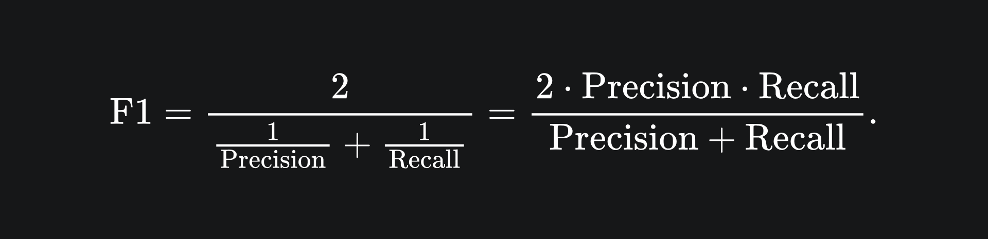
Namely, the F1 score is the harmonic mean of precision and recall. We can also write the F1 score formula terms of TP, FP and FN:
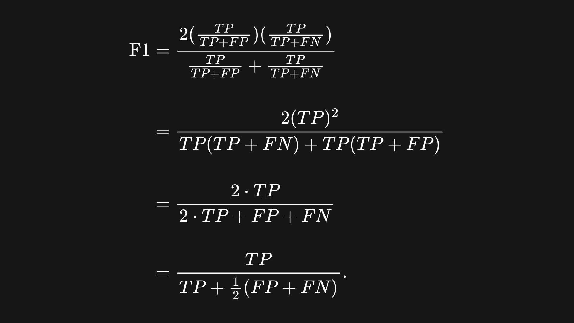
We can see that the F1 score suffers when the arithmetic mean of FP and FN is high. In particular, it doesn’t suffice to only minimise one of FP or FN.
Overall, the F1 score is a useful metric when dealing with imbalanced datasets.
Small caveat
It seems as though there isn’t a global consensus on which way around the predicted values and actual values should be displayed on the confusion matrix. In this article, I have put the predicted values on the rows and the actual values on the columns. Basically, be careful when looking on online sources, as some may use the transpose of my depiction.
Packing it all up
No algorithms unpacked this week, I’m afraid. But performance metrics are super important for the sake of evaluating your model’s performance in a way that is conducive towards your prediction goals. I hope that this article has helped shed some light on the subtleties that need to be considered when it comes to model evaluation. Now, a brief summary as always:
Accuracy tells you the proportion of data points that were correctly classified by the model. This metric is not well-suited to datasets containing class imbalance.
Recall: represents the proportion of actual positive data points that were predicted as positive. Ideal for when you want to minimise the number of positive results that slip past the model. Recall concerns the first column of the confusion matrix.
Precision: represents the proportion of predicted positive data points that were actually positive. Ideal for when you want to minimise the number of incorrect positive predictions made by the model. Precision concerns the first row of the confusion matrix.
The green and red highlighting used in the below animation helps me to remember which way around recall and precision go on the confusion matrix:
Training complete!
I hope you enjoyed reading as much as I enjoyed writing 😁
Do leave a comment if you’re unsure about anything, if you think I’ve made a mistake somewhere, or if you have a suggestion for what we should learn about next 😎
Until next Sunday,
Ameer
PS… like what you read? If so, feel free to subscribe so that you’re notified about future newsletter releases: