Solving the Multi Armed Bandits problem with the Successive Elimination algorithm

Eliminating sub-optimal arms with the help of Hoeffding's Inequality.

Hello fellow machine learners,

Last week, we introduced reinforcement learning with the Multi Armed Bandit problem. Be sure to read that article before this one, as we’ll be building on those ideas:

This time round, we will think about our arm-pulling game through the lens of uncertainty, the basis upon which reinforcement learning is fundamentally intertwined.

Let’s get to unpacking!

Empirical mean rewards

We will continue with our discussion of Gaussian bandits. That is to say, the rewards sampled from arm i follow a Gaussian distribution of mean μ_i and standard deviation σ_i. These parameters are unknown to the player.

Here is a brief recap of the mathematical framework we set up last week. The only difference we will make here is to extend the discussion to n arms rather than just three.

Using i to index the arms, and t to index the rounds of play, let:

• A_t denote the player’s arm choice at round t. So in the context of n levers, A_t takes a value in {1, 2,…, n} for each value of t.

• X_t denote the reward received at round t (this will be distributed following the corresponding Gaussian arm).

• μ_i denote the mean reward of arm i. We also let i* denote the index of the optimal lever, with corresponding optimal mean reward set as μ*=μ_i. Recall that you as the player do not know the value of i*: the aim is to figure this out with a good enough strategy.

We also add the following definitions. Let:

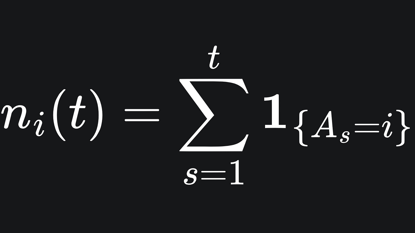
• n_i(t) represent the number of times that arm i is played up to round t:

  

• Consider the arm A_i, for i fixed. We let μ̂_i,t denote the empirical mean reward from arm i by the end of round t. This is what we as the player believe the average reward is from arm i based on the rewards we have accumulated from it during our play:

  

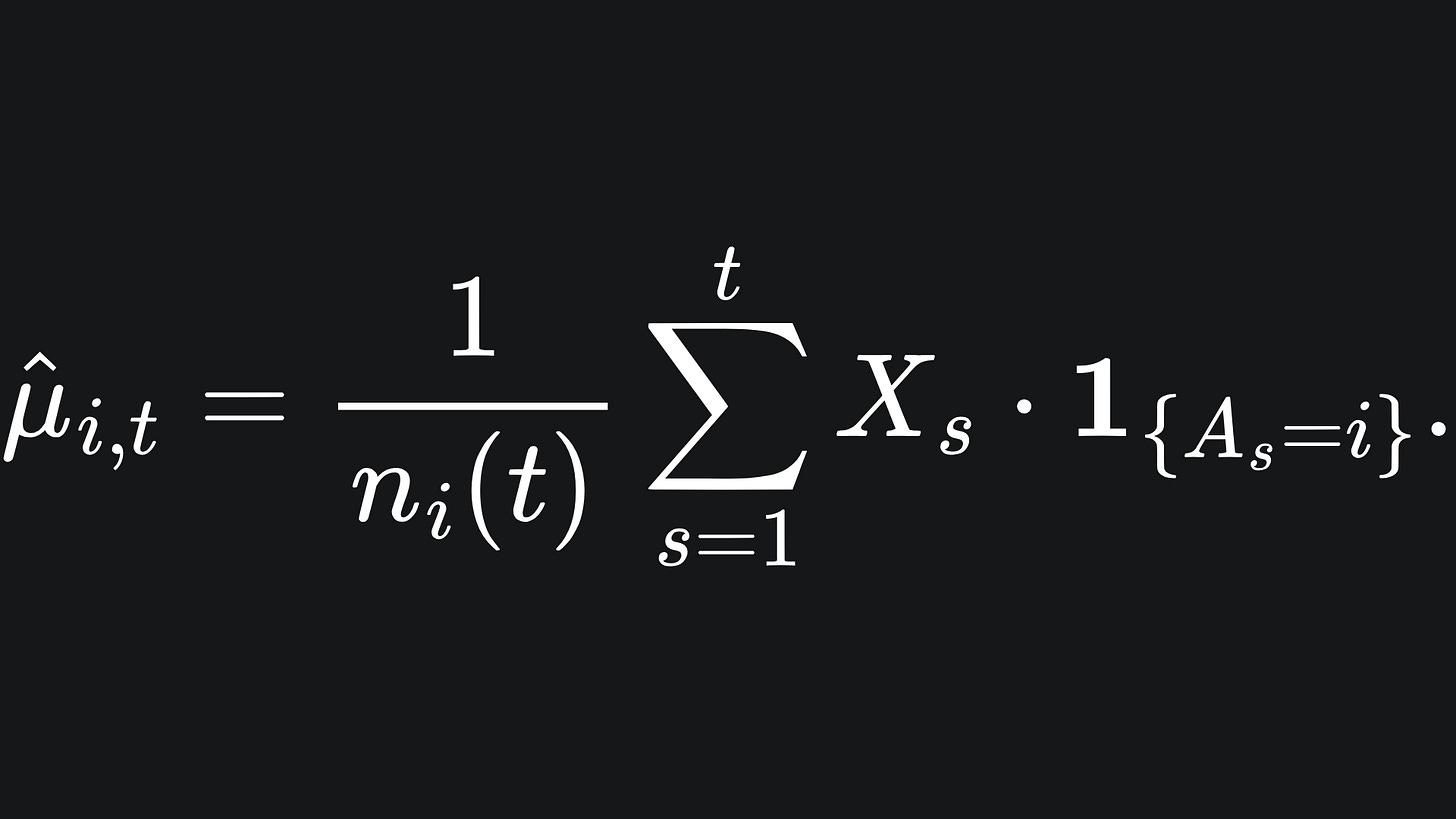
  (The indicator function in the above summation ensures that we only sum up rewards from arm i in these t rounds.)

  🚨 Important point 🚨

  The empirical mean reward, despite the use of the word ‘empirical’, is actually a random variable. This is because it is the average of the random variables X_i, which themselves are sampled at random from a Gaussian distribution.

  The expression n_i(t) is also a random variable, because it counts the occurrences of the {A_s=i}, an inherently stochastic quantity.

How do we use all this to estimate the true mean reward from arm i, μ_i? Intuitively, you would want to play arm i lots of times and average out the result. This intuition is imprinted in the theory of statistics by the Law of Large Numbers. The more times we pull arm i, the more confidence we have in estimating the value of μ_i, which in maths looks like:

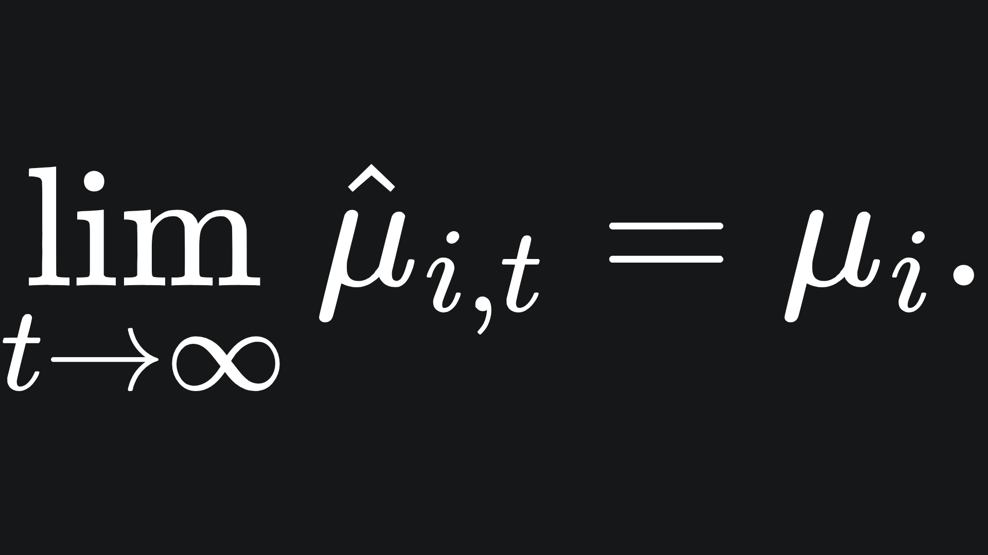
The more times we pull arm i, the more confidence we have in our estimate for the value of μ_i. In reality though, we can’t necessarily play with the arms an arbitrarily large number of times. Or at least, we hope to explore whether there are more efficient methods to find out such information.

Gaussian tail bounds

We will continue with our discussion of Gaussian bandits. That is to say, the rewards sampled from arm i follow a Gaussian distribution of mean μ_i and standard deviation σ_i.

The nice thing about Gaussian random variables is that we know a lot about the spread of their values from their parameters. The larger the variance, the more widespread the values are. We can frame the decay of the Gaussian pdf with concentration inequalities:

We state the following concentration inequalities¹:

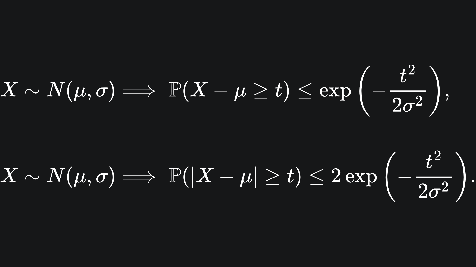
This inequality tells us how far away a realised value of X is likely to be from the mean of the distribution from which X is drawn. The larger the value of t, the smaller the right hand side of the inequalities.

We can derive more complicated expressions from these tail bounds with the help of Hoeffding’s inequality.²

For example, in the context of our bandit problem, we have for a fixed arm i that

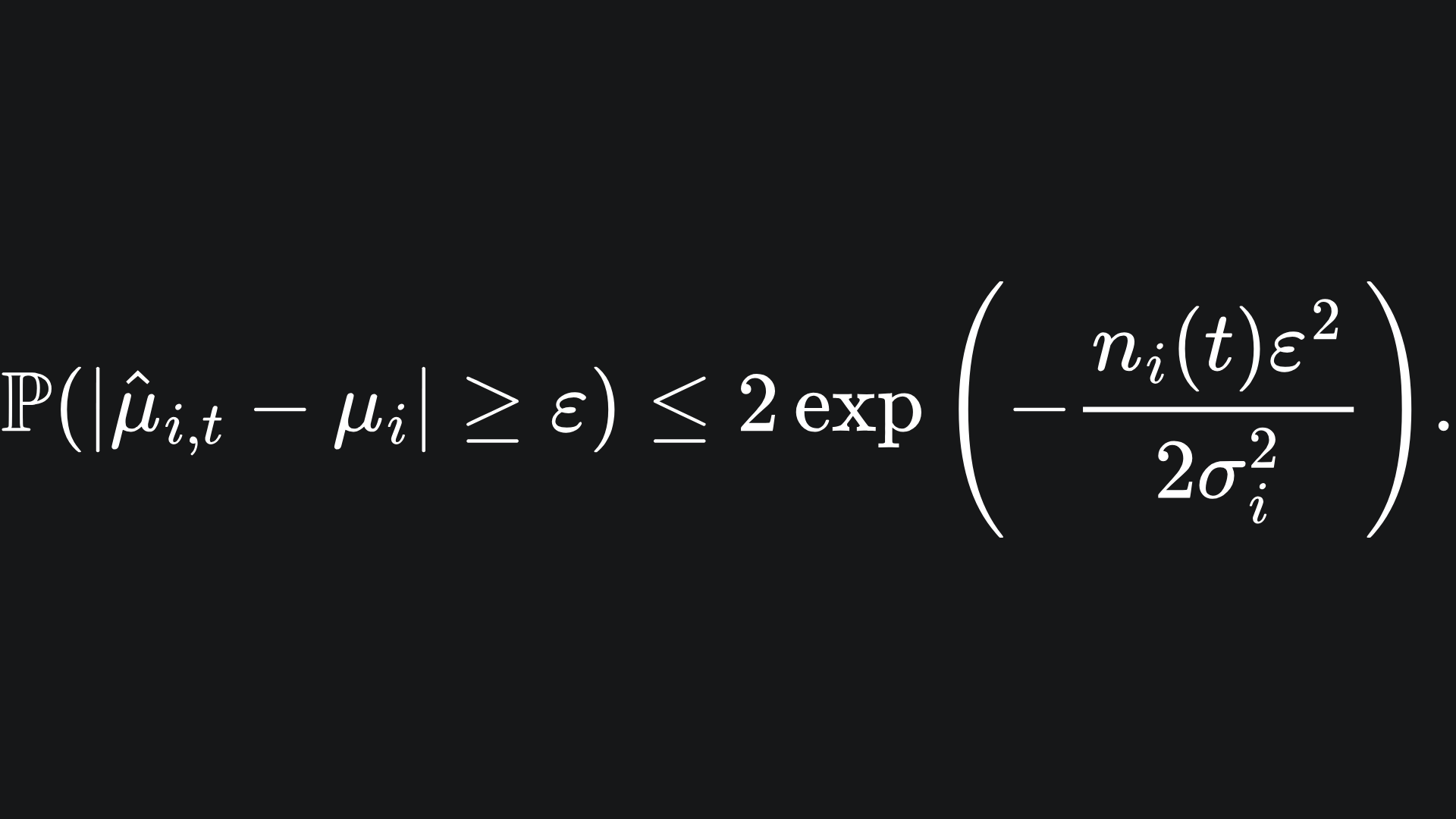
The value of ε is arbitrary. By setting the right hand side equal to δ and rearranging to remove the ε, this becomes³

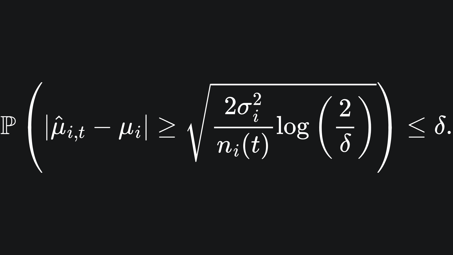
What does this mean? This is saying that, with probability δ, the empirical mean reward will not be sufficiently close to the true mean reward. It will help our understanding to take the complement of the event:

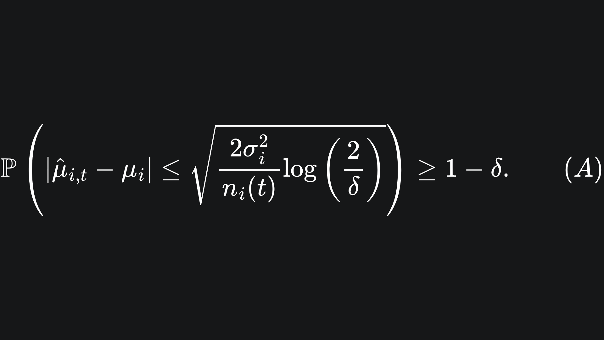
So if δ takes a small value, then with high probability (WHP), we have that the empirical mean reward will be sufficiently close to the true mean reward.

We are resorting to the use of confidence intervals like this, because we require some means of quantifying how close the empirical mean rewards are to the true mean rewards for each arm. The corresponding probability is controlled by the parameter δ.

We will call the ugly-looking square root expression the confidence radius for arm i by the end of round t:

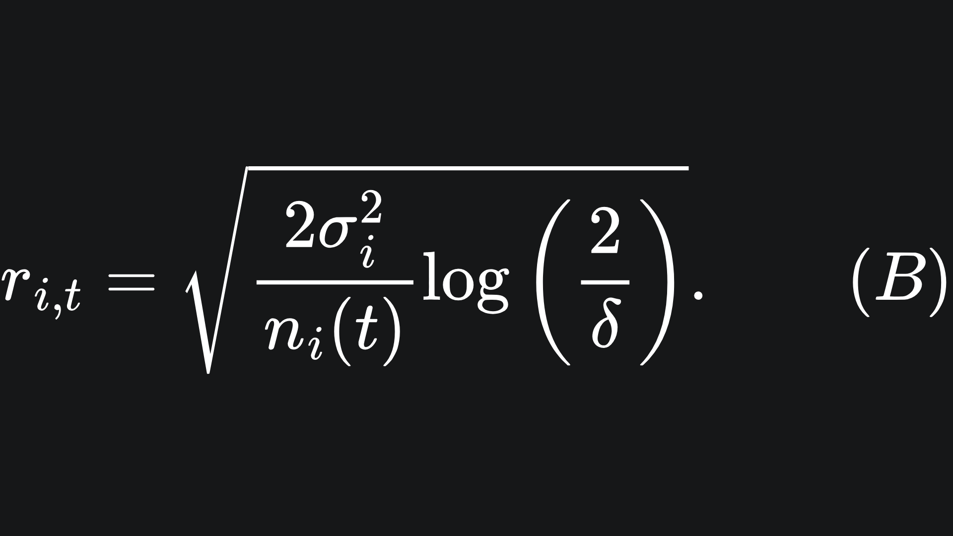
This looks complicated, but the maths should align with our intuition of how to situation changes when the parameters are adjusted:

💡 The smaller the value of δ, the more sure we are of the closeness of our empirical mean reward to the true mean reward as given by inequality (A). However, the corresponding confidence radius is larger (δ term in the denominator of the logarithm). This makes sense; we can be more sure of the empirical value being within a larger interval.

💡 The more times we pull arm i, the more sure we can be that the empirical reward is close to the true mean reward. This is exemplified in equation (B); the confidence radius decreases for larger values of t.

Successive elimination

The epsilon-greedy algorithm aimed to find the most optimal arm by alternating between exploration and exploitation. In each exploitation round, the arm with the largest empirical mean reward was pulled. However, sub-optimal arms were not eliminated at all during any exploration round. If there were a way to eliminate the (observed) sub-optimal arms through the algorithm’s runtime, then the procedure would be more robust against poor arm choices.

This is where the successive elimination algorithm comes in. Here is how it works:

👣 We break the MAB game up into ‘phases’. In each phase, we will play each arm the same number of times.

👣 After each phase, we compute the empirical mean reward for each arm and analyse the corresponding confidence intervals. Since we are playing every arm in each phase, n_i(t) = t for each arm i, where t is the current phase count.

👣 We will eliminate any arm whose confidence interval lies strictly below the confidence interval of any other arm.

👣 We then enter the next phase and repeat until only one arm remains.

Here is a video explaining the details:

Do take a look at the code I put together (link here) to better understand how the algorithm works under the hood.

Will we always be left with one arm?

You may have wondered this as you read the final step of the algorithm outlined in the previous section.

This depends heavily on the reward distributions of the arms. We may not be able to reduce down to just one arm if the true mean rewards of the arms are sufficiently close together, the confidence intervals are large enough and we are working with a finite number of phases.

Packing it all up 📦

That wraps things up for our second Multi Armed Bandit algorithm.

Here is the usual roundup:

💡 The successive elimination algorithm aims to reduce the set of arms in play by eliminating arms whose empirical mean reward confidence intervals lie below those of any other arm. This helps to keep the SE algorithm more robust versus, say, the epsilon-greedy algorithm.

💡 We have to use confidence intervals here, because we cannot guarantee that the empirical mean reward of each arm are exactly the same as the corresponding true mean rewards, which arise from the underlying Gaussian distributions. This is where Hoeffding’s inequality comes into play, allowing us to stipulate the closeness of the empirical and true values “with high probability (WHP)”.

💡 The success of the successive elimination algorithm depends on the number of rounds being played, the choice of δ and how close the Gaussian distributions are.

Training complete!

I hope you enjoyed reading as much as I enjoyed writing 😁

Do leave a comment if you’re unsure about anything, if you think I’ve made a mistake somewhere, or if you have a suggestion for what we should learn about next 😎

Until next Sunday,

Ameer

PS… like what you read? If so, feel free to subscribe so that you’re notified about future newsletter releases:

Sources

• My GitHub repo where you can find the code for the entire newsletter series: https://github.com/AmeerAliSaleem/machine-learning-algorithms-unpacked

• “Action Elimination and Stopping Conditions for the Multi-Armed Bandit and Reinforcement Learning Problems”, by Eyal Even-Dar, Shie Mannor and Yishay Mansour: https://www.researchgate.net/publication/220320322_Action_Elimination_and_Stopping_Conditions_for_the_Multi-Armed_Bandit_and_Reinforcement_Learning_Problems

• “Reinforcement learning: An Introduction”, by Richard S. Sutton and Andrew G. Barto: https://web.stanford.edu/class/psych209/Readings/SuttonBartoIPRLBook2ndEd.pdf (^ btw this is a GOATed resource for RL in general)

• “Bandit Algorithms”, by Tor Lattimore and Csaba Szepesvari: https://www.cambridge.org/core/books/bandit-algorithms/8E39FD004E6CE036680F90DD0C6F09FC

• Lecture notes on sub-Gaussian random variables: https://ocw.mit.edu/courses/18-s997-high-dimensional-statistics-spring-2015/a69e2f53bb2eeb9464520f3027fc61e6_MIT18_S997S15_Chapter1.pdf

1. The study of Gaussian tail bounds comes from concentration inequalities with so-called ‘sub-Gaussian random variables’. Check the final bullet point in the ‘Sources’ section.

2. We won’t be going into this here, but again, check the sources for more!

3. I encourage you to try this substitution and rearrangment for yourself.