
Loss functions for ML regression models
Mean Squared Error, Mean Absolute Error and the Huber loss.

Hello fellow machine learners,
We are continuing our discussion of loss functions. Make sure you’ve checked out last week’s post before jumping into this one, as we’ll be borrowing similar concepts and notation:
As the title suggests, loss functions don’t just exist for classification models: they also appear for regression models! In this article, we’ll discuss some examples and draw some comparisons between them.
Once you’ve done your pre-reading1…
…let’s get to unpacking!
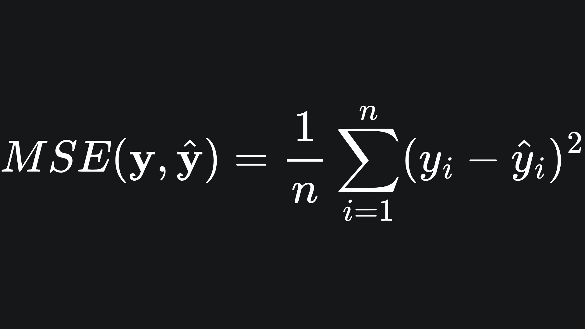
Mean Squared Error
The Mean Squared Error (MSE) takes the squared difference between the true and predicted labels:
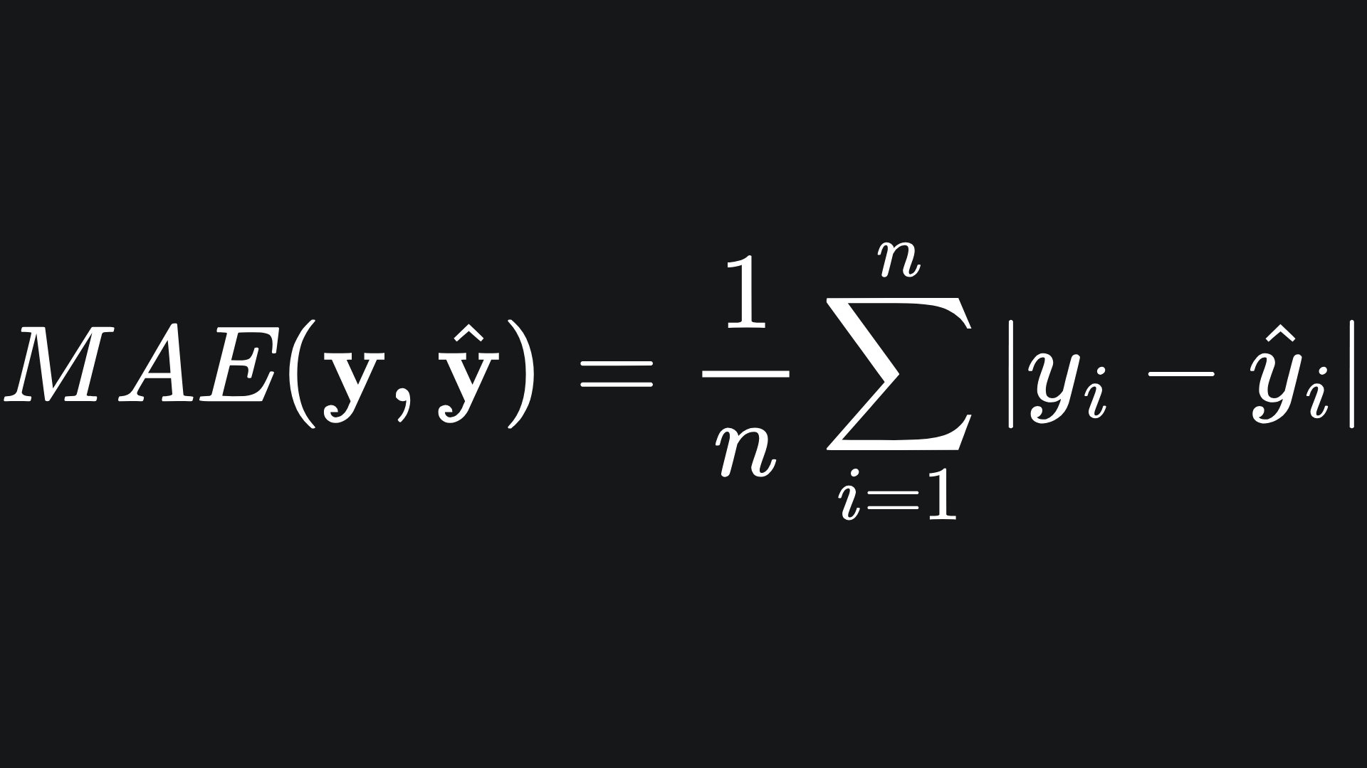
Mean Absolute Error
As the name suggests, the Mean Absolute Error (MAE) takes the absolute difference between the true and predicted labels:
As a side note, when computing differences, we should at least take either the squared difference or the absolute difference. If this is not intuitive to you, check out this article I wrote a while back.
Why use squared error over absolute error?
MAE seems a bit simpler, right? Taking the correct +/- sign is less computationally demanding than squaring values, especially when there are large values and/or many data points involved.
Well, for one thing, the MAE is not a smooth function. This is an issue we mentioned last week that we’ll return to in due course. For now though, trust me when I say that it’s better for us to have smooth loss functions due to the fact that they are differentiable. The MSE doesn’t have this problem, since it’s a nice ol’ reliable quadratic.
For another, the MSE is more sensitive to outliers. This is evident when comparing the two functions on the same plot:
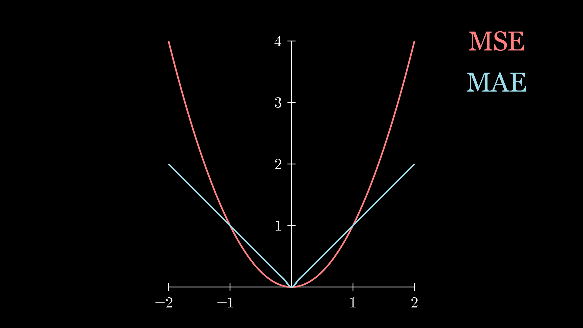
We can see that, for large input values, the MSE has a bigger value. This will happen when the model tries to fit for outliers; chances are that the deviation between the predicted and true label will be large. However, note that, for values between 0 and 1, the MSE has smaller values than MAE. This is because the product of two fractions is a value smaller than either constituent.
The MSE’s outlier sensitivity can be a benefit or a hindrance depending on your use case:
😄 If you’re building a regression model to predict house prices, it may be important to capture the patterns of really expensive and really cheap properties. These two extremes can be thought of as outliers, but they both have a role to play in general real estate data.
☹️ If you’re building a regression model to predict a patient’s testosterone levels based on other biological factors, there could be patients who just happen to have very high (of very low) levels of the hormone naturally, be it through genetics or otherwise. These outlier values could disrupt the model’s ability to generalise, in which case the MAE would be a better suited loss function.
Huber loss
If only we could have both the smoothness of MSE and the outlier robustness of MAE…
…oh wait, we can! Enter the Huber loss:
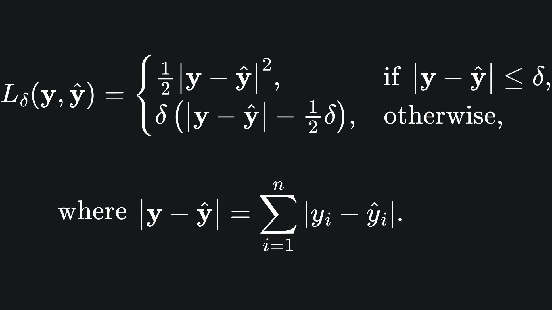
It looks rather complicated, so let’s break it down:
💡 For values of |y-ŷ| smaller than the parameter δ, the Huber loss takes on a quadratic shape. This allows for a smooth turning point in the Huber loss curve, resolving the issue at zero for MAE.
💡 For values of |y-ŷ| smaller than δ, the Huber loss takes on a form similar to standard MAE. We subtract the quadratic term in δ at the end to ensure continuity of the Huber loss function at the point where |y-ŷ|=δ.
💡 The δ parameter controls the threshold of where we change between quadratic behaviour and linear behaviour.
Let’s see what the Huber loss looks like for different values of δ:
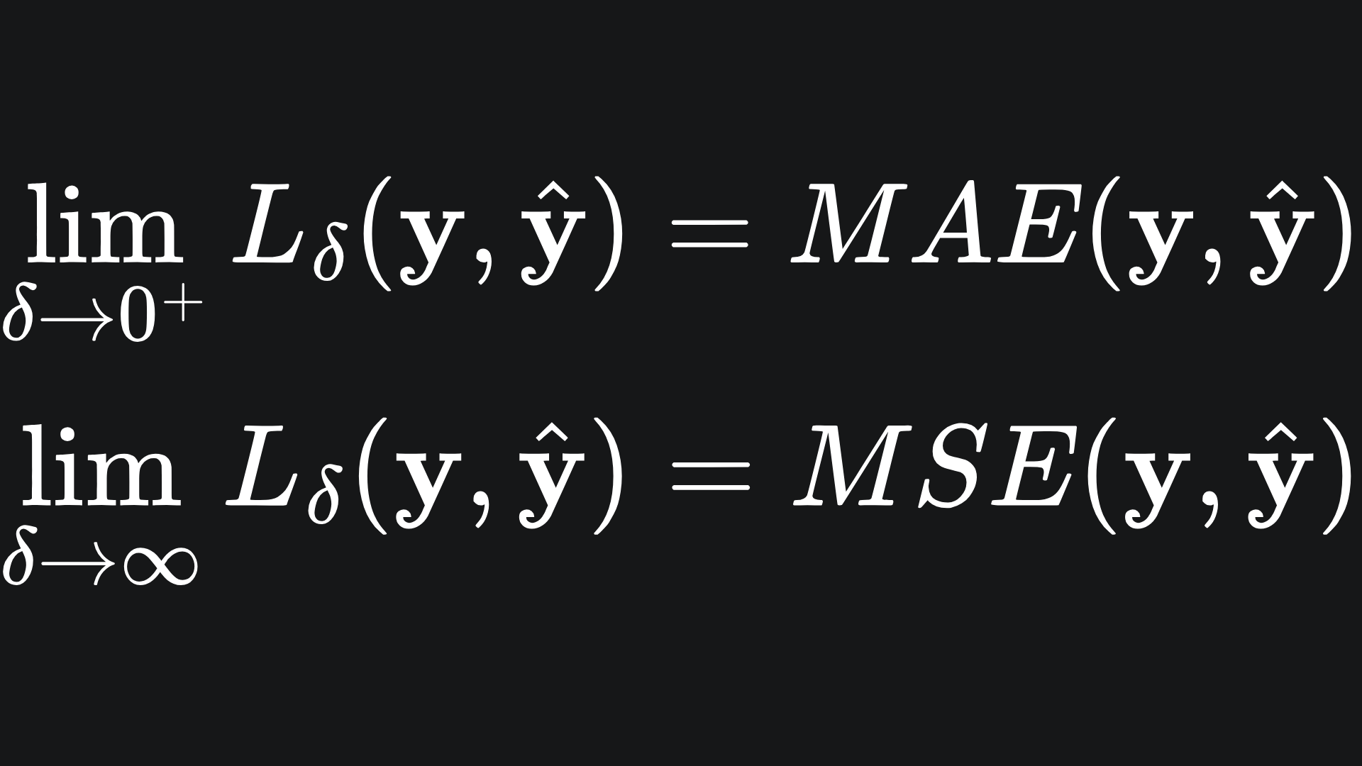
The smaller the value of δ, the more the Huber loss resembles MAE, and vice versa for larger values of δ. Mathematically, we can consider what happens in the limit:
What value of δ should I choose?
This is yet another question that we’ll return to later on. But the idea is that δ controls the size of the gradient for the Huber loss. This is something that you’d want control over when training models with respect to the goal of minimising loss. But more on that soon enough.
Packing it all up
And that’s a snapshot of loss functions for regression models! Over the past two weeks, we’ve covered some essential foundations that will bring us to some exciting ML concepts. But slow and steady wins the race.
It’s summary time:
📦 The Mean Squared Error scales the difference between the true and predicted label quadratically. This makes the loss function sensitive to outliers, the utility of which depends on your regression context.
📦 The Mean Absolute Error simply takes the absolute difference between the true and predicted labels. While more robust to outliers than MSE, the MAE is not a smooth function, and so isn’t differentiable.
📦 The Huber loss combines the MSE and MAE, with the dominance of either loss function controlled by the δ parameter.
Training complete!
I hope you enjoyed reading as much as I enjoyed writing 😁
Do leave a comment if you’re unsure about anything, if you think I’ve made a mistake somewhere, or if you have a suggestion for what we should learn about next 😎
Until next Sunday,
Ameer
PS… like what you read? If so, feel free to subscribe so that you’re notified about future newsletter releases:
Sources
My GitHub repo where you can find the code for the entire newsletter series: https://github.com/AmeerAliSaleem/machine-learning-algorithms-unpacked
Or not. Your call, I guess…