
Explaining word embeddings with word2vec, CBOW and Skip-gram
Exploring how computers can store words in vector form, and how word2vec allows for the construction of meaningful word embeddings.

Hello fellow machine learners,
Last time, we discussed bidirectional Recurrent Neural Networks, and showed how they are able to better capture sentence contexts compared to the standard RNN architecture. You won’t need that stuff today, but do check it out if you’re interested:

Today, I would like to take some time to explain how computers interpret words. As with anything in machine learning, computers simply don’t have a built-in understanding for anything other than numerical digits. For example, computers think of images as collections of pixels, with each defined by numbers for either greyscale saturation or RGB colouring1.
The goal of this article is to explain not only how words can be numerical encoded, but also why the encodings are meaningful, i.e. they preserve word context in some way.
Let’s get to unpacking!
Word embeddings
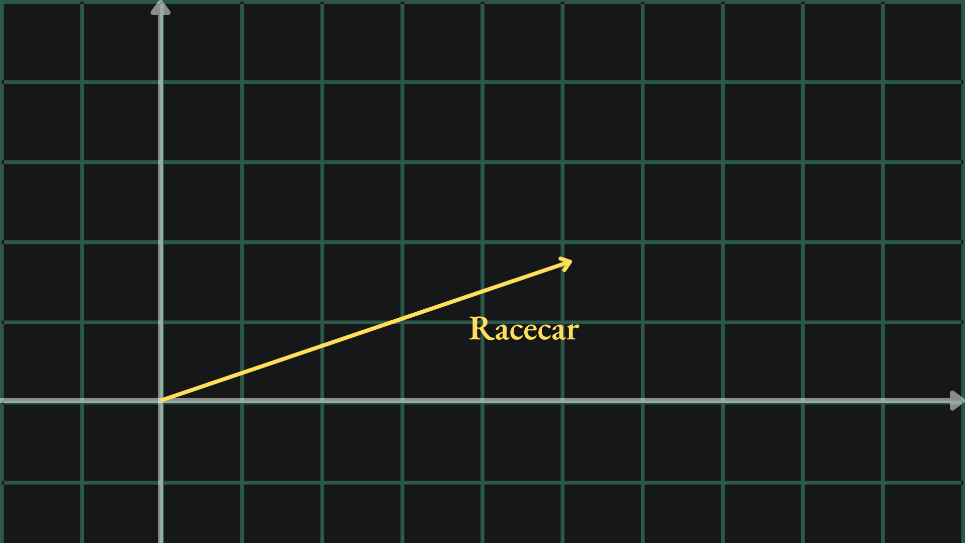
As mentioned before, computers don’t understand words the same way we humans do. They require English words to be modified into numbers. A useful representation would be that of a numerical vector. We could take a word like “racecar” and transform it somehow into, say, a vector in two dimensions with its own magnitude and direction:
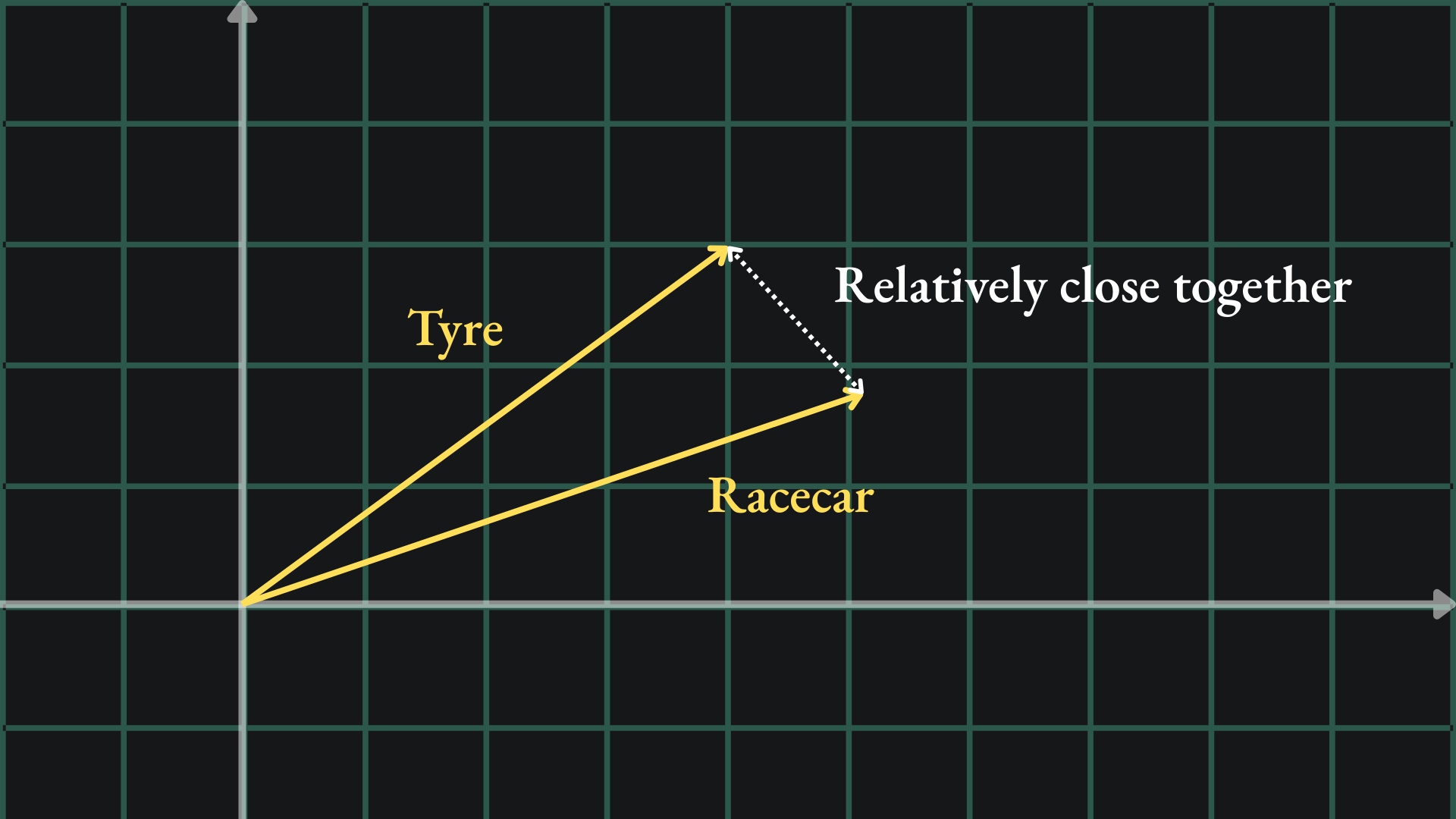
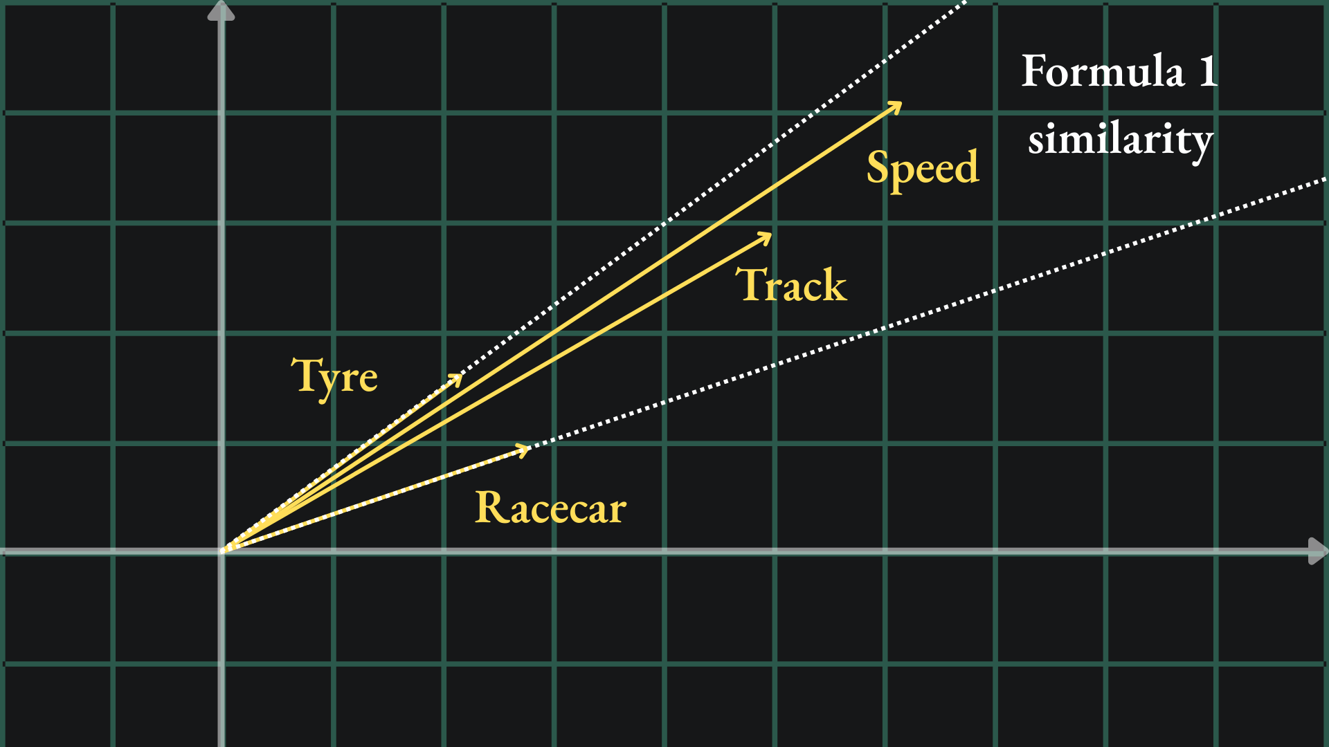
This is called a word embedding- we take a word and embed it into a higher dimensional space. Crucially though, we want to ensure that words with similar meanings are embedded in a similar way. Since the words “tyre” and “racecar” are both related to cars, we might want their embeddings to be close together in our new space:
As you might imagine, there exist methods to create embeddings from text data. One such example is word2vec. According to the TensorFlow docs:
word2vec is not a singular algorithm, rather, it is a family of model architectures and optimisations that can be used to learn word embeddings from large datasets.
(Don’t worry, we’ll talk more about word2vec later in this article.)
The TensorFlow embedding projector allows us to visualise word embeddings. The default mode shows a sample of 10,000 word2vec embeddings. These embeddings are actually in 200-dimensional space in their raw form. But on this webpage, Principal Component Analysis (PCA)2 is applied to each embedding, which acts to ’project’ them down into just three dimensions so that we can view them.
Don’t just take my word for it though- have a play around with the embedding projector yourself! You can select an individual point and isolate the plot to consider a fixed number of its neighbours.
Cosine similarity
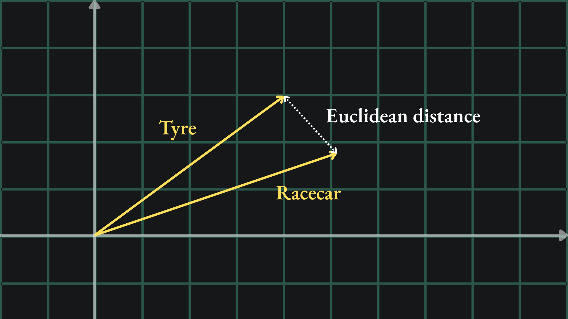
What does it actually mean for a pair of word embeddings to be ‘close’ to one another?
The most intuitive way of measuring this would be to measure the Euclidean distance between the two vectors. At school, you would use a ruler to measure the distance between the tips of the vectors:
Another way to measure distance is with the cosine similarity. For a pair of vectors, this metric looks at the angle between the vectors rather than comparing their lengths. The formula is given by
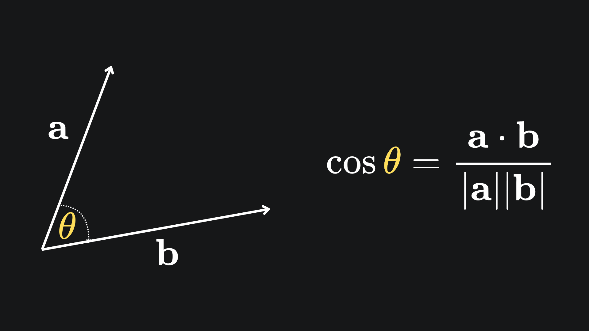
The dot product is defined as
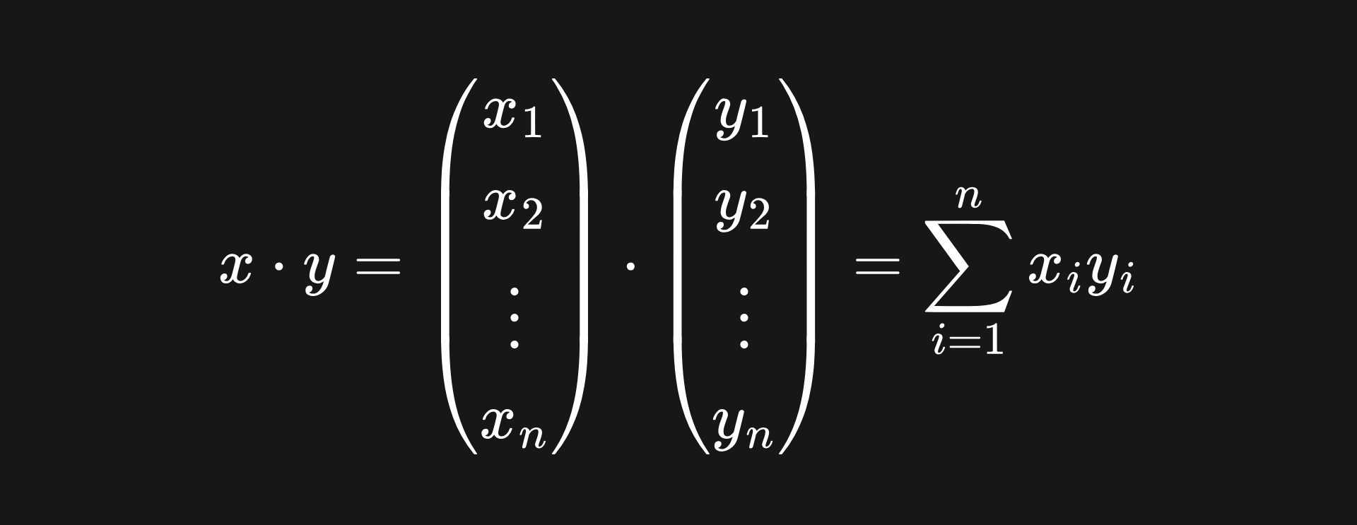
(If you’d like to learn a bit more about vectors and the dot product, check out this article I wrote in early 2025.)
I have summarised the main qualities (and hence usefulness) of cosine similarity in the below image:
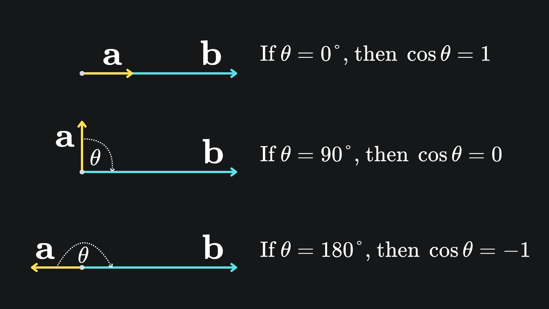
Essentially, any embeddings that align in the same direction are considered similar, whilst those that align in different directions are considered dissimilar. This allows us to embed multiple similar words in the same direction, even if the vectors are assigned different magnitudes in the embedding space:
word2vec
With all that said, how do we assign embeddings such that similar words are kept close together in our embedding space?
The original word2vec paper explains two simple neural network approaches that can be used to learn good word embeddings for a given input corpus3.
Let’s start with a small example. Consider the sentence “You should subscribe to my Substack”. The aim is to create 2D word embeddings for each of the six words.
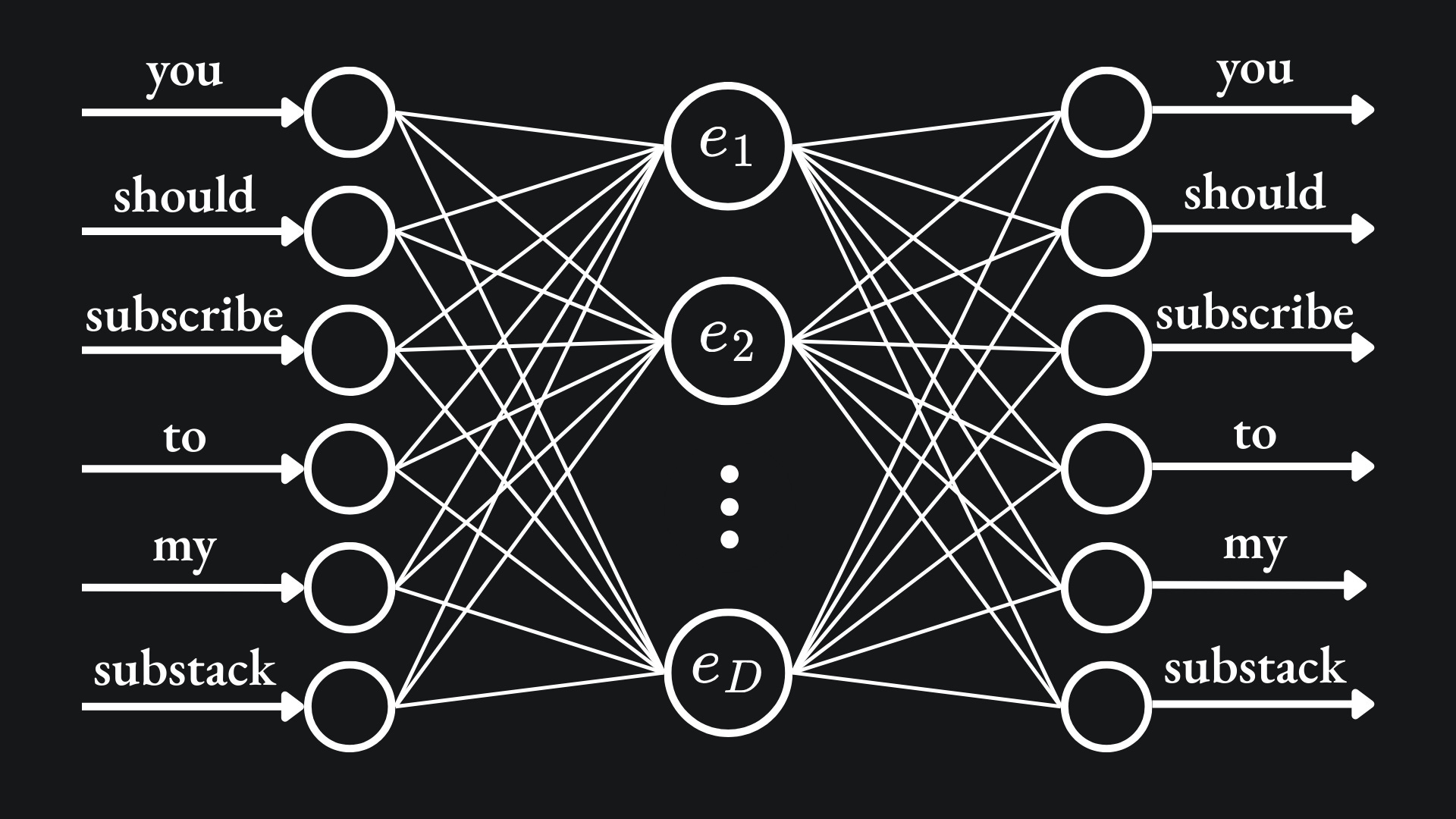
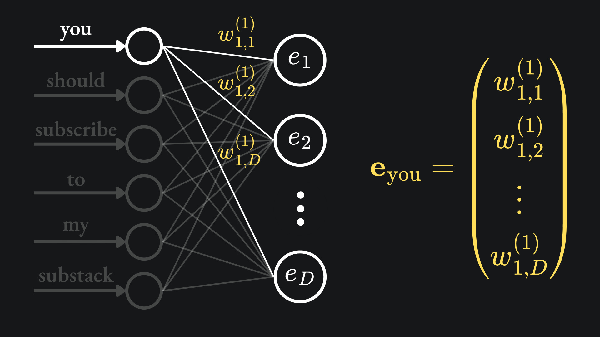
The network architecture proposed by the paper is comprised of a hidden layer of D neurons, with both the input and output layer having V neurons. The value D corresponds to the embedding dimension size, while V refers to the network’s vocabulary size. So for my toy example, this would be a network with V=6 neurons in the input layer, D=2 in the hidden layer and V=6 neurons in the output layer:
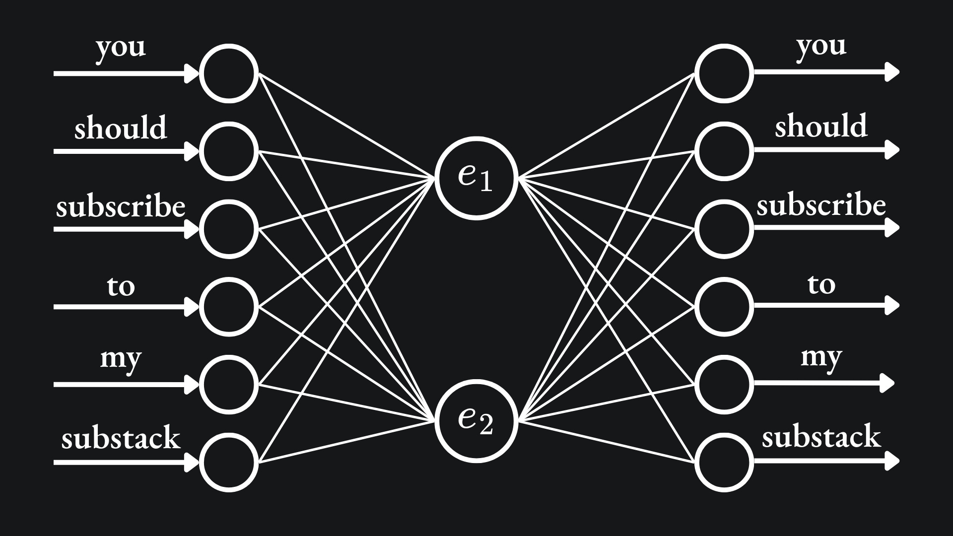
The weights between the input and hidden layers give us the word embeddings we want. For example, the weights on the pair of edges connecting the first input node to the hidden layer constitute the word embedding of the word ‘you’:
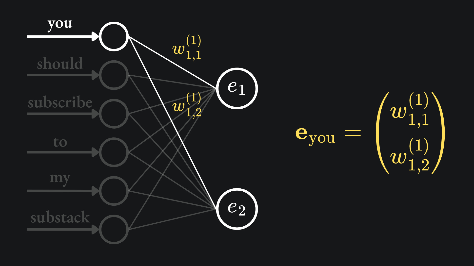
Note that the weights of the edges between the hidden layer and output layer don’t contribute directly to the embeddings, but are still responsible for shaping the network output. The network outputs are created by combining the values from the hidden layer and passing them through the SoftMax activation function.
Continuous Bag-Of-Words (CBOW)
The first model described in the word2vec paper is the Continuous Bag-Of-Words (CBOW) model. For a given target word, the network is presented with the N words before and after it in the sentence, with the aim of predicting the target word.
For the case where the target word is “subscribe” with D=2, the network is presented with the words “you”, “should”, “to” and “my”4:
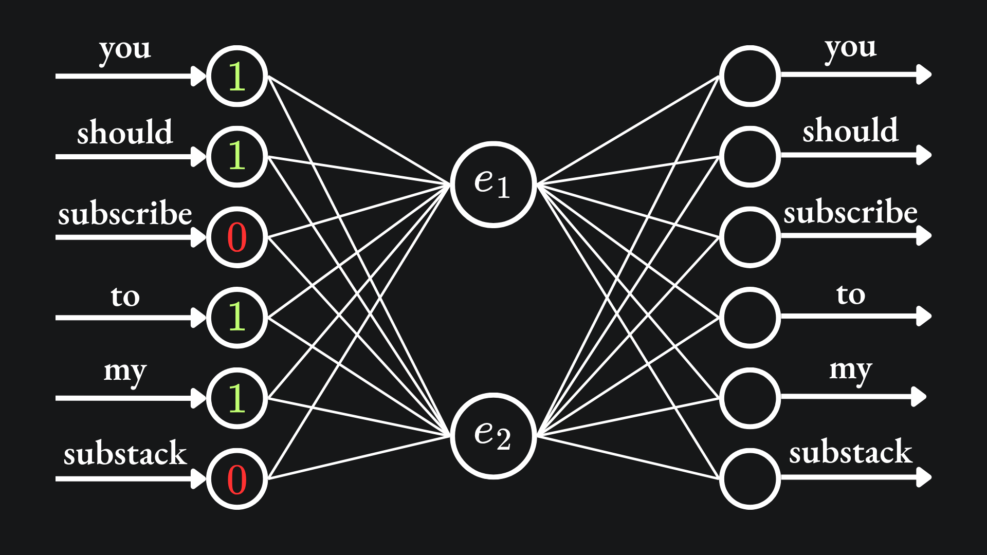
The goal is for the SoftMax output to align the most with the output corresponding to the word “subscribe”:
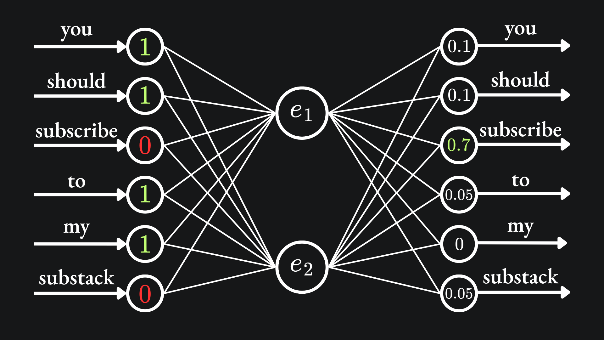
In this example, the input-output training example can be thought of as ([“you”, “should”, “to”, “my”], “subscribe”). When numerically encoded, the input looks like (1,1,0,1,1,0) and the output looks like (0,0,1,0,0,0).
This procedure is applied to the different choices of target word. And as with any regular neural network, we apply the forward pass of training data, compute the loss of the network and then update the weights through the backpropagation procedure. The goal is for the network to learn meaningful weights, hence meaningful word embeddings! I think that this is pretty cool; by setting up the network architecture like this, good word embeddings are an immediate consequence of a well-trained neural network.
If you wanted to increase the dimension of the embedding space, then you can add more neurons to the hidden layer. So the case of embedding dimension D>2 may look like the following:
As before, the word embedding for the word “you” comes from all the weights between the first node of the input layer and the hidden layer’s nodes:
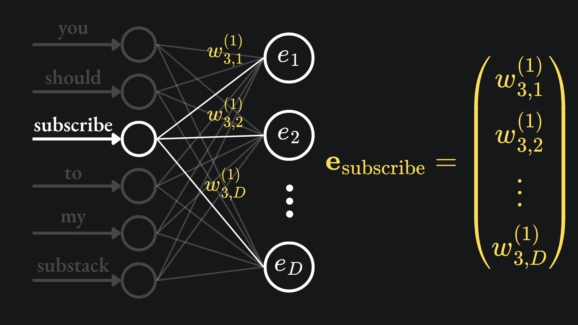
Finally, here is where the word embedding for the word “subscribe” comes from, just to sink the point in:
Continuous Skip-gram model
The other model mentioned in the word2vec paper works in a similar manner to CBOW. But rather than predicting a word using its neighbours, the continuous Skip-gram model uses the word in the middle to predict what its neighbours are.
Let’s suppose that the input word here is “subscribe”, and we aim to predict the C=2 words before and after the word. Then the network input (encoded) is just (0,0,1,0,0,0), and we hope that the network provides large SoftMax signals at the first, second, fourth and fifth indices:
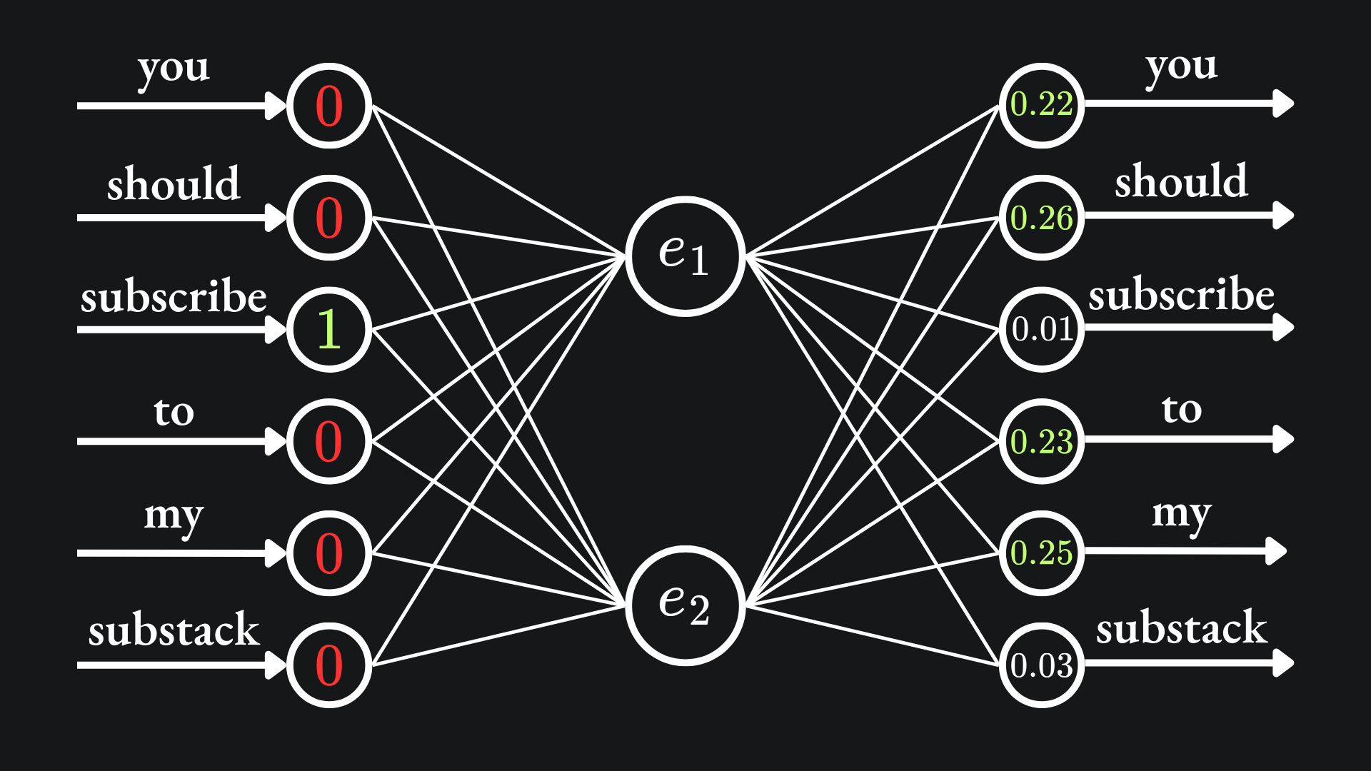
The word2vec paper remarks that the larger the value of C, the higher the quality of the resultant weights, albeit at the expense of computational complexity.
Static embeddings
So that’s how word2vec works. There are similar examples to word2vec, such as GloVe, which you can read more about here.
One major limitation of these approaches, however, is that they produce static embeddings. That is to say, once an embedding has been created for a given word, it cannot be changed.
Let’s try and motivate why this might be an issue. Recall the initial example of the ‘tyre’ and ‘racecar’ word embeddings:

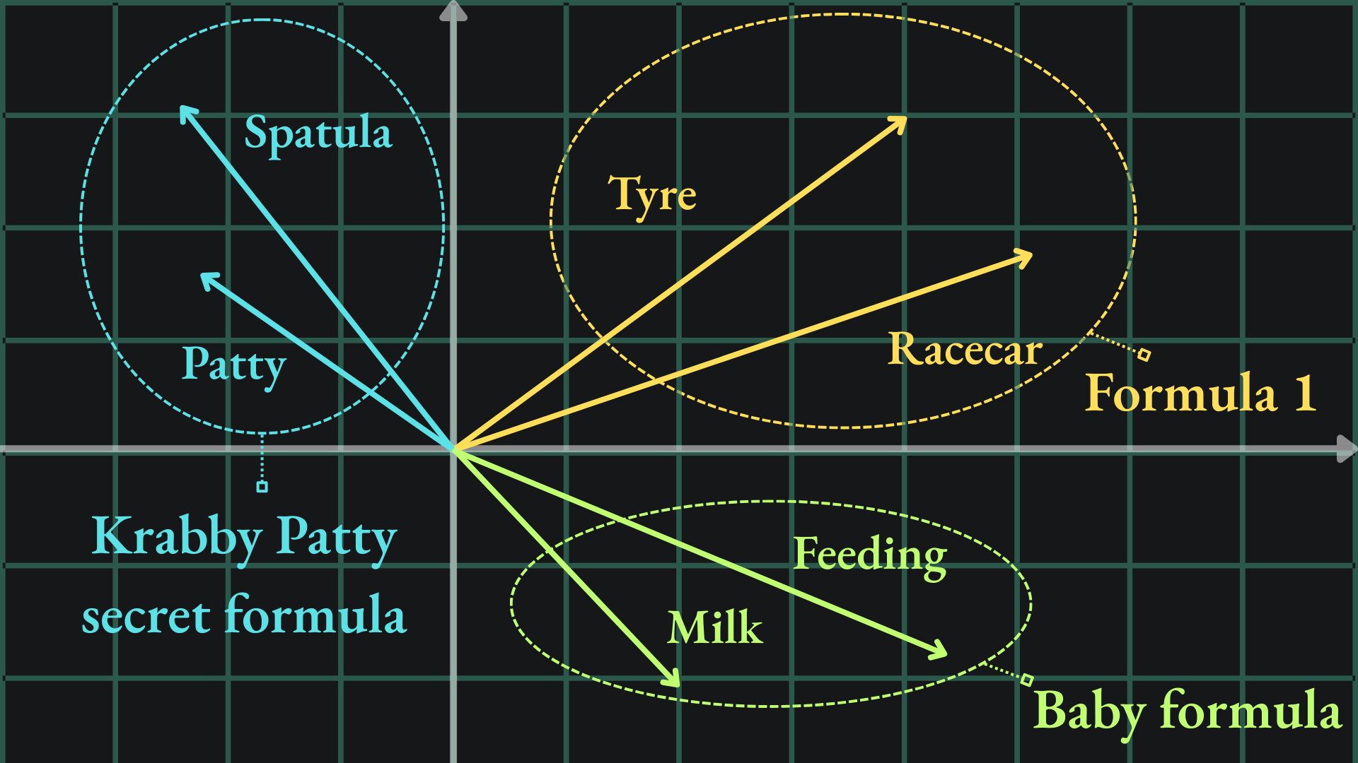
We might want the word “formula” to be close to these two vectors in this embedding space too. You know, because of Formula 1. However, the word “formula” could also refer to a mathematical formula, baby formula, or even the Krabby Patty secret formula, all of which mean quite different things. It may be difficult to capture all of these contrasting meanings with one word embedding.
One solution is to implement an embedding space of much larger embedding dimension: 100 dimensions, or maybe even 10,000 dimensions? This could allow the word “formula” to maintain closeness to multiple semantic fields5 at once, especially when using cosine similarity as the metric of choice over the Euclidean distance. The problem with this lies in the curse of dimensionality. The more dimensions used for the embedding space, the more network parameters. According to the word2vec paper, the training complexity of both CBOW and Skip-gram is directly proportional to the embedding dimension D. Is there a way to solve our problem by avoiding the inflation of D?
Here’s an idea: we establish all of our word embeddings in one space, and then make modifications to the embeddings as we get more context of the situation. By “modifications”, I mean the use of vector addition/subtraction to move them around in the embedding space. Focussing on the word “formula” again: if we realise at some point that the context is motorsport racing, then the “Formula 1” meaning makes sense, and so we ought to have our word embedding close to words like “tyre” and “racecar” as mentioned before. On the other hand, if we’re talking about a certain absorbent, yellow and porous fellow, then the word “formula” should be moved closer to, say, “spatula”, “patty” and suchlike.
The original word2vec paper was published by a team of Google researchers in 2013. That was a while ago6, and the landscape for handling text data with ML has changed drastically since then.
In future articles, we’ll discuss dynamic embedding techniques, i.e. embeddings that are not fixed and can be updated in line with the sentence context.
Packing it all up
There is more to the word2vec paper that I haven’t covered here, such as in-depth comparison between these models and RNN architectures. I’d recommend that you have a read.
Anyway, here is the usual roundup:
📦 The cosine similarity provides a measure of closeness of vectors by orientation rather than physical distance. This allows us to embed multiple similar words in the same direction, even if the vectors are assigned different magnitudes in the embedding space.
📦 The word2vec paper from 2013 proposes two neural network models, CBOW and Skip-gram, that each produce word embeddings from network weights. I think that this is pretty cool; by setting up the network architecture like this, good word embeddings are an immediate consequence of a well-trained neural network.
📦 A limitation of such approaches is that they produce static embeddings. That is to say, once an embedding has been created for a given word, it cannot be changed. Cutting-edge architectures are capable of using dynamic embeddings, that are flexible enough to change through sentential context.
Cheeky bonus
Some potentially useful word definitions in the context of Natural Language Processing, which I included in various footnotes:
Corpus: “a collection of written texts, especially the entire works of a particular author or a body of writing on a particular subject.”
Semantic field: “a lexical set of semantically related items, for example verbs of perception.”
Lexical: “relating to words or vocabulary of a language.”
Training complete!
I hope you enjoyed reading as much as I enjoyed writing 😁
Do leave a comment if you’re unsure about anything, if you think I’ve made a mistake somewhere, or if you have a suggestion for what we should learn about next 😎
Until next Sunday,
Ameer
PS… like what you read? If so, feel free to subscribe so that you’re notified about future newsletter releases:
Sources
My GitHub repo where you can find the code for the entire newsletter series: https://github.com/AmeerAliSaleem/machine-learning-algorithms-unpacked
The word2vec paper, “Efficient Estimation of Word Representations in Vector Space”, by Mikolov, Chen, Corrado and Dean: link
“GloVe: Global Vectors for Word Representation”, by Pennington, Socher and Manning: link
More on greyscale images, and more on coloured images respectively.
PCA is an unsupervised learning technique that I never got round to discussing in 2025. Let me know in the comments if you want me to write about it at some point!
Corpus: “a collection of written texts, especially the entire works of a particular author or a body of writing on a particular subject.”
NB the paper remarks that the use of four previous and four future words resulted in the best performance. I am using just two previous and two future words here to help illustrate the concept.
Semantic field: “a lexical set of semantically related items, for example verbs of perception.” Lexical: “relating to words or vocabulary of a language.”
To put this into perspective, I started secondary school in 2013!