Backpropagation explained with examples

Gradient descent, partial derivatives and the chain rule. Get your pen and paper at the ready! And maybe a few different colours too...

Hello fellow machine learners,

Last week, we really went to town on activation functions, the functions which provide us the means to model non-linear patterns with neural networks. Nice!

This time round, we’ll discuss the process by which a neural network’s weights and biases are updated (aka how a neural network learns): backpropagation.

I would strongly recommend you catch up on my previous two articles if you haven’t already:

🔐 An introduction to what neural networks are can be found in Neural Networks 101

🔐 Be sure to check out Introducing non-linearity in neural networks with activation functions (it does what it says on the tin)

When I first learned about backpropagation in neural networks, I made the mistake of jumping straight into the mathematical theory without looking at simpler numerical examples. I puzzled for hours (maybe even days) over the theorems and formulas that governed the technique.

But have no fear! We won’t be going through backpropagation from this perspective. Rather, we’ll discuss how backpropagation works by applying it to network architectures we’ve explored in previous articles.

Here’s the thing though- backpropagation is just the use of the chain rule a bunch of times. That’s it.

The issue is that the notation can get really confusing, especially for larger networks that have lots of parameters. But I think the key is to focus on smaller, more manageable examples first.

And in order to demonstrate that…

…let’s get to unpacking!

Backpropagation

The aim of backpropagation is to equip the neural network with the weights and biases that will minimise the corresponding loss function value.

The loss function will be written with respect to the network’s output for the given network input value(s). But we know from previous weeks that at its core, the output prediction is just a function of the neural network’s weights and biases. So our loss function can indeed be written with respect to the model parameters too. And we want to minimise the loss, in particular minimising it with respect to these parameters.

Gradient descent

This minimisation process an be achieved with gradient descent. Recall that gradient descent takes the form

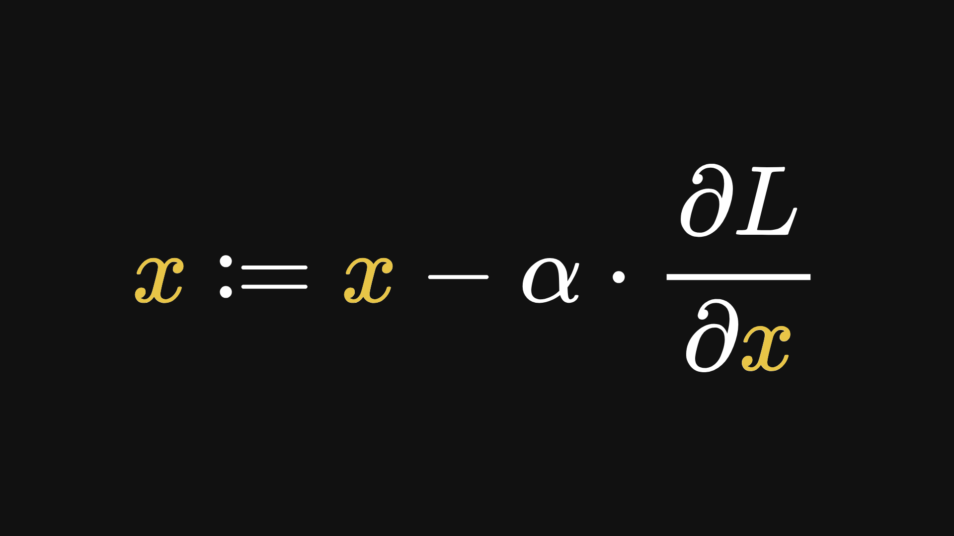
where α is the learning rate. The larger the learning rate, the larger the step taken at each iteration of the algorithm. This doesn’t necessarily mean that the minimisation happens faster though; if these steps are too large, then the algorithm could easily skip past a minimum point.

Conversely, a smaller learning rate yields smaller steps in gradient descent. If the learning rate is too small though, then the algorithm might take too long to converge, or could even get stuck in a local minimum.

Here is a general way to express the desired use of gradient descent for the parameters of a neural network:

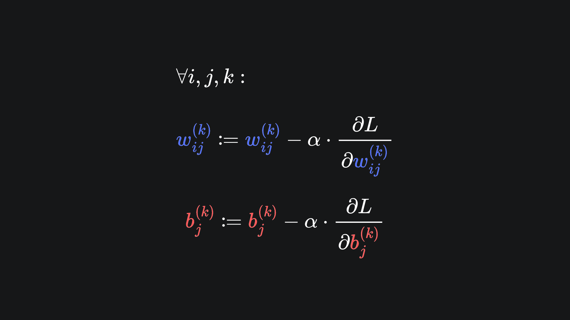
You can think of this as the application of a separate gradient descent algorithm to each network parameter. Crucially though, we want to compute all these updates simultaneously:

Let’s make this notion concrete with the simple example of a neural network of two weights, one bias and one sigmoid activation function:

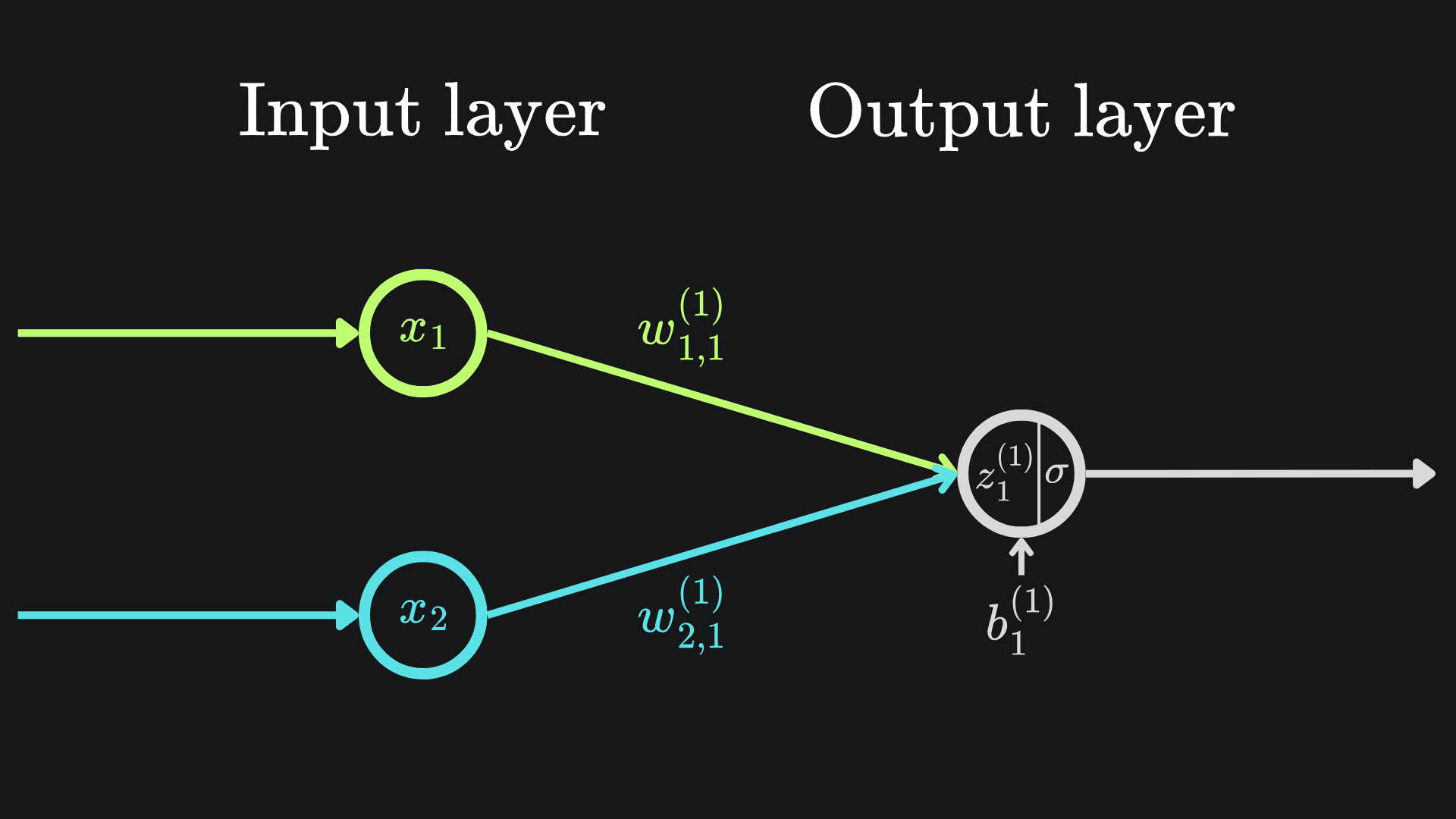
Don’t forget that σ(z₁⁽¹⁾) = a₁⁽¹⁾. This is final output prediction of the neural network in question.

Chain rule

Our goal is to find the partial derivative of the loss with respect to w_1,1⁽¹⁾, w_2,2⁽¹⁾ and b₁⁽¹⁾. Taking the loss as the Mean Squared Error, we have by the chain rule that

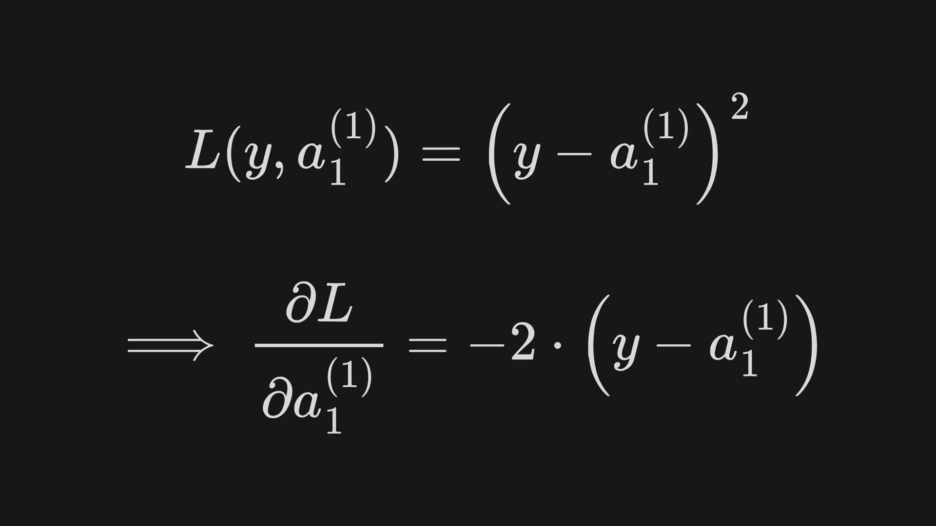
(Note that this looks like just a regular Squared Error rather than the Mean Squared Error, but that’s just because we have a scalar predicted label rather than a vector of predicted labels.)

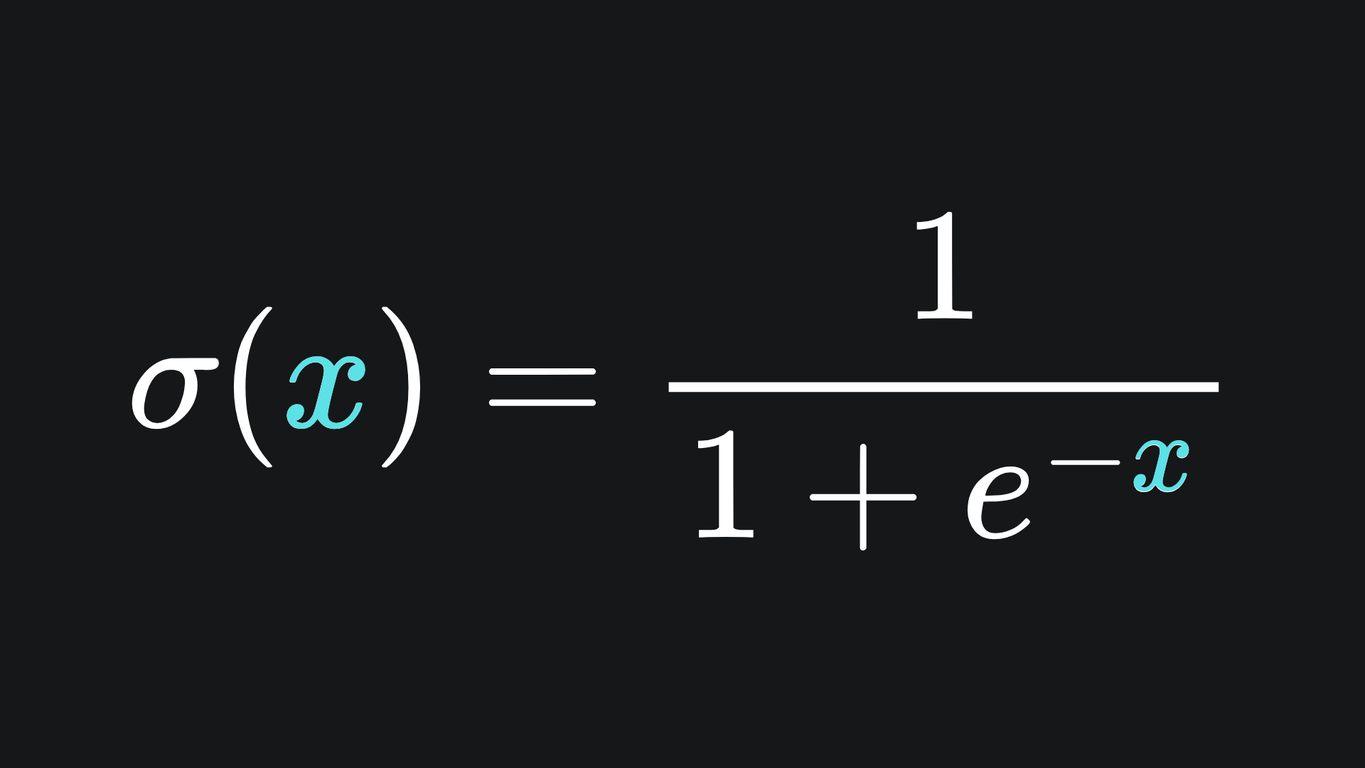
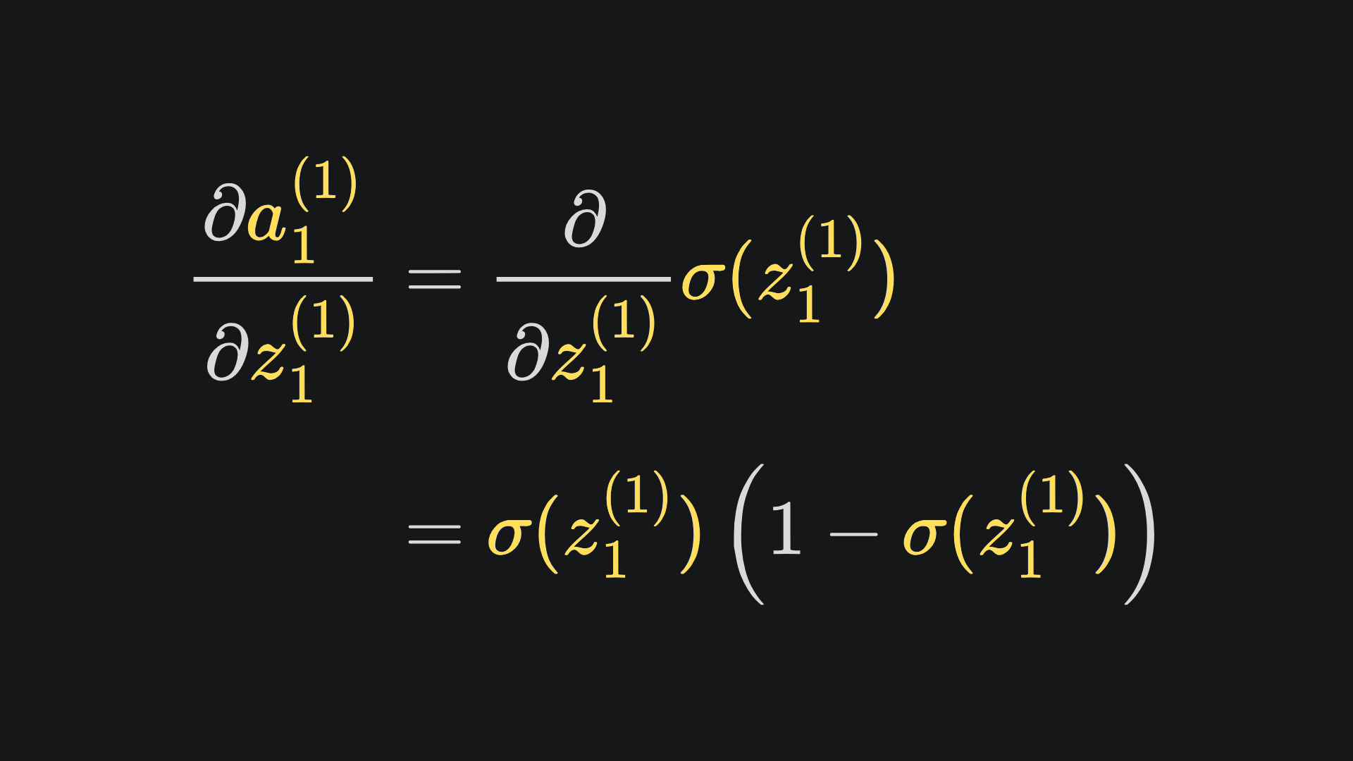
Here we have that a₁⁽¹⁾ = σ(z₁⁽¹⁾). Recall from last week that the sigmoid function is defined as

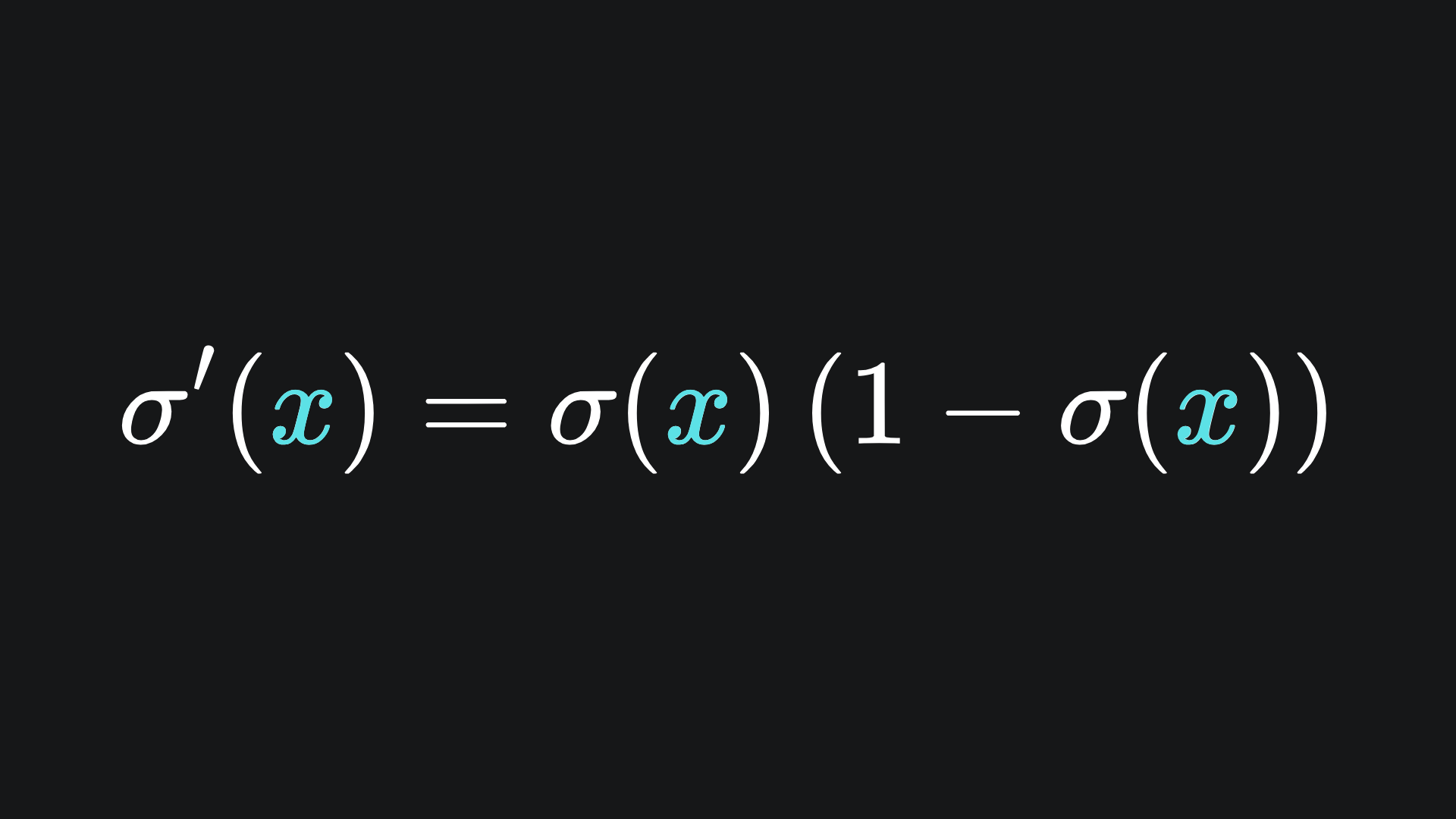
with derivative

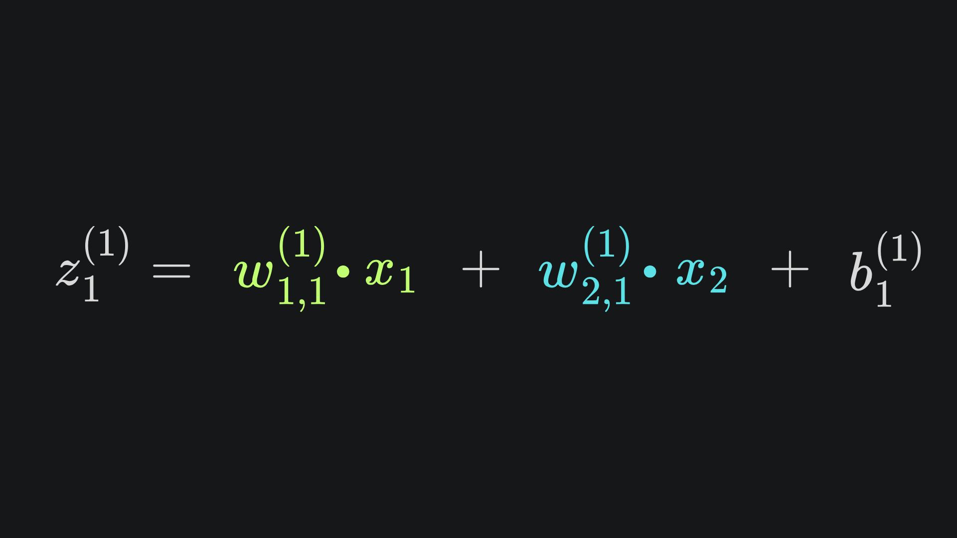
According to the neural network diagram, we know that z₁⁽¹⁾ is a linear combination of w_1,1⁽¹⁾, w_2,2⁽¹⁾ and b₁⁽¹⁾:

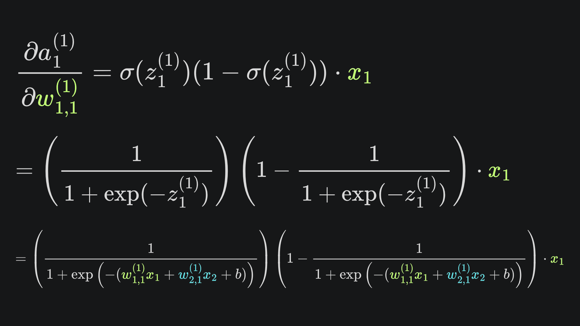
Applying the chain rule again, we have

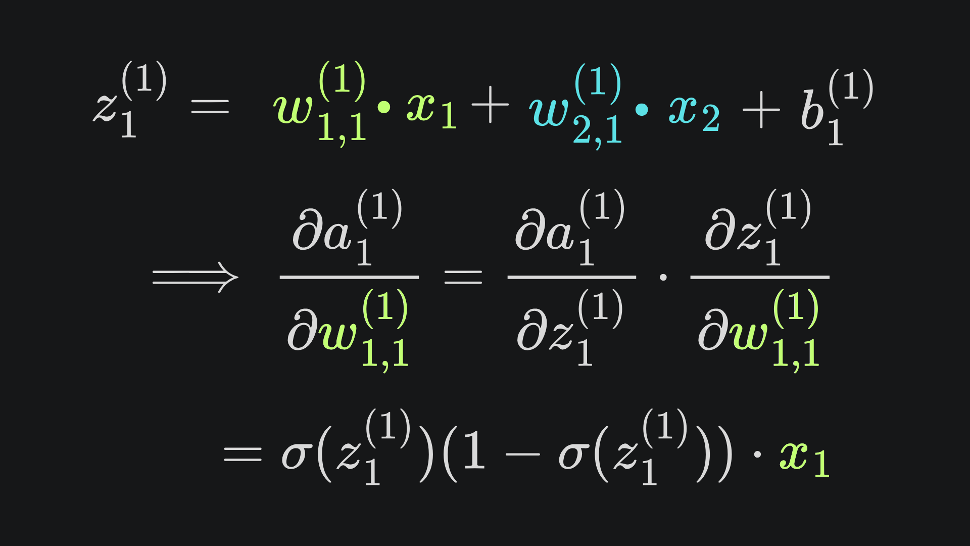
If you want the full explicit form of the partial derivative, then here you go (but don’t say I didn’t warn you):

Fortunately, the other two partial derivatives follow super similar formulations. Here are the three results together, written in ‘z form’ for brevity:

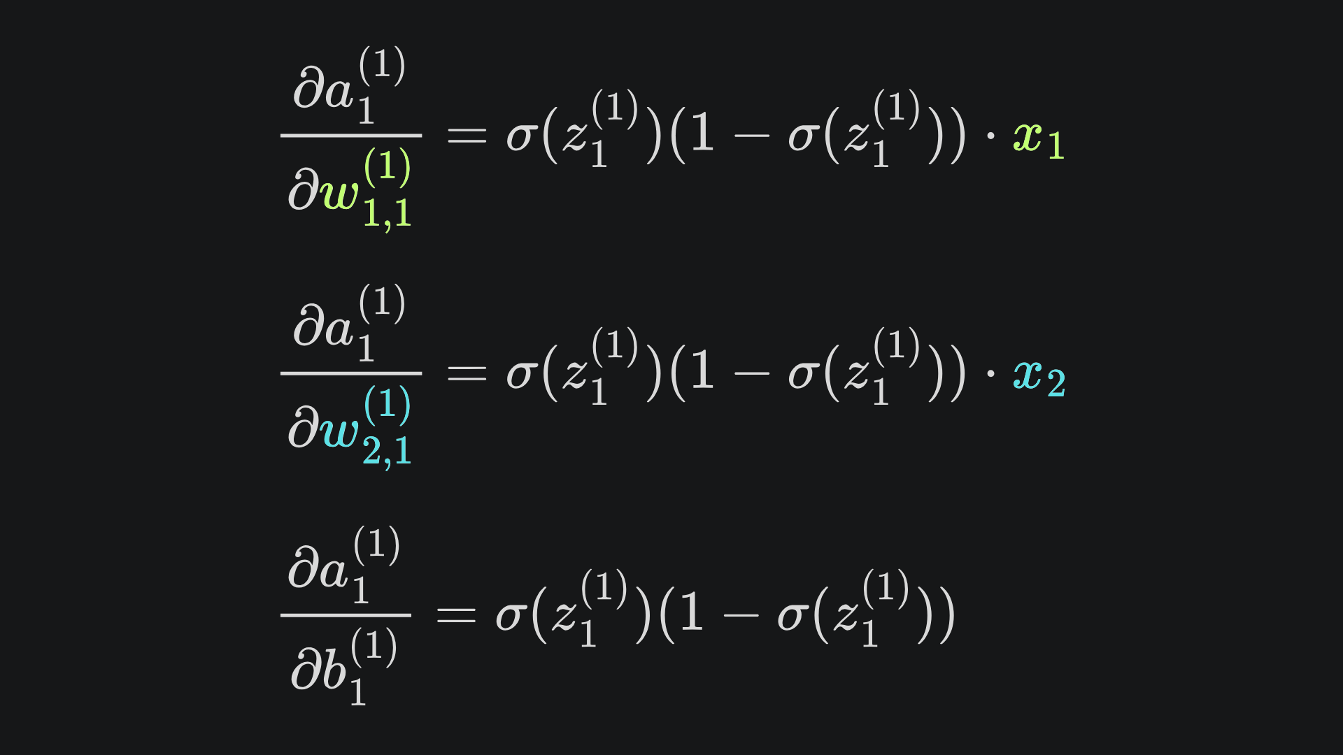
As you can hopefully see, it’s mainly an exercise in applying the chain rule and substituting values.

To clarify:

💡 Start by (randomly) initialising the weights and bias.

💡 Apply forward propagation to generate a network output given input data.

💡 Apply gradient descent to modify the weights and bias in the hopes of minimising the loss.

💡 Rinse and repeat 👏🏼

If that all makes sense so far, then read on!

A more complicated example

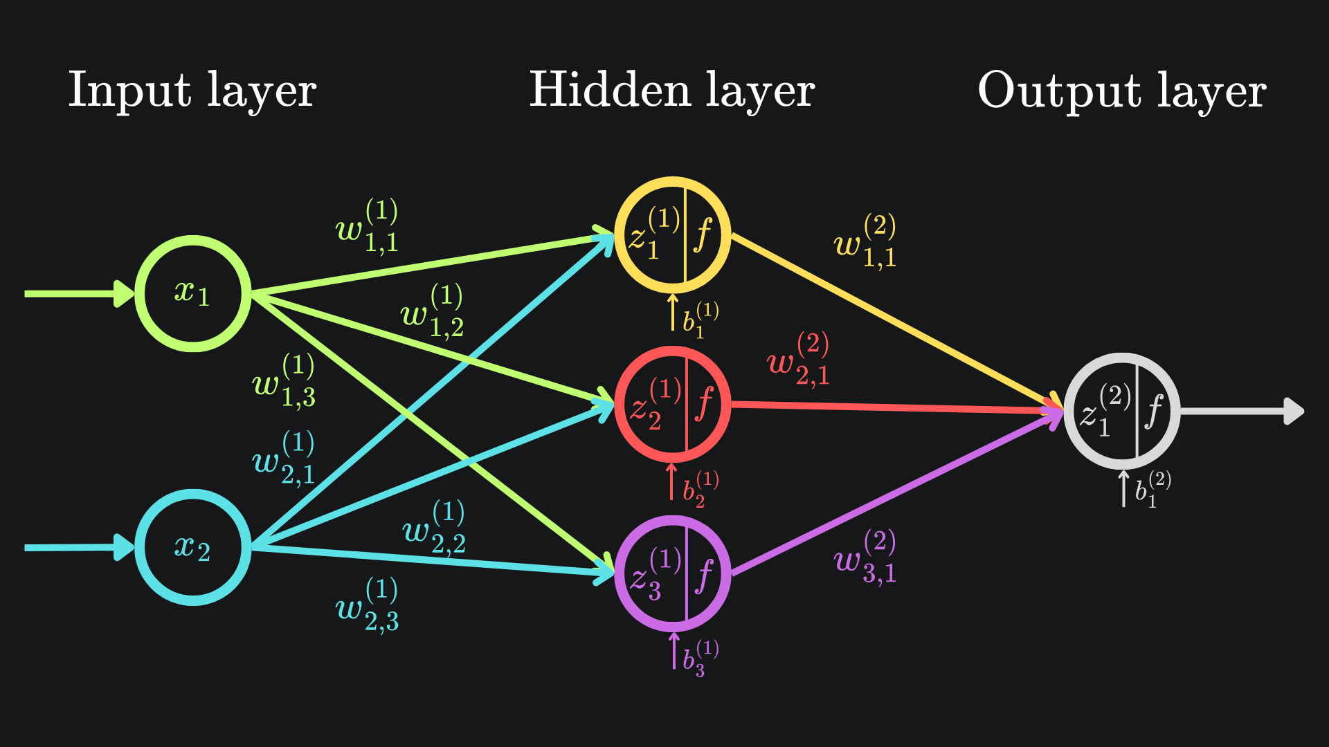
Time to step things up:

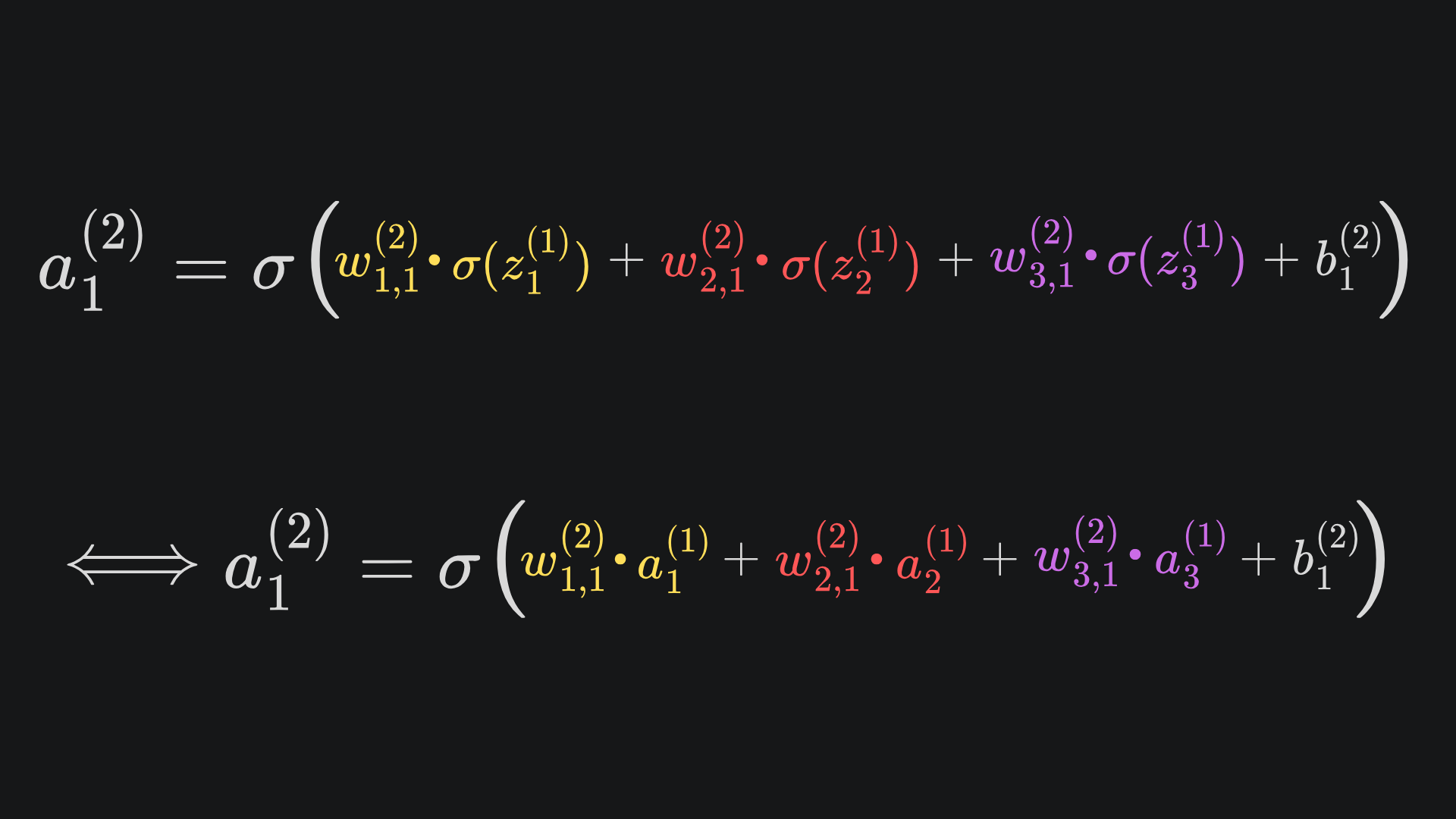
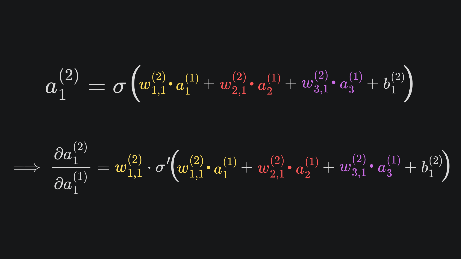
Recall from last week that the neural network’s output value a₁⁽²⁾ is given by

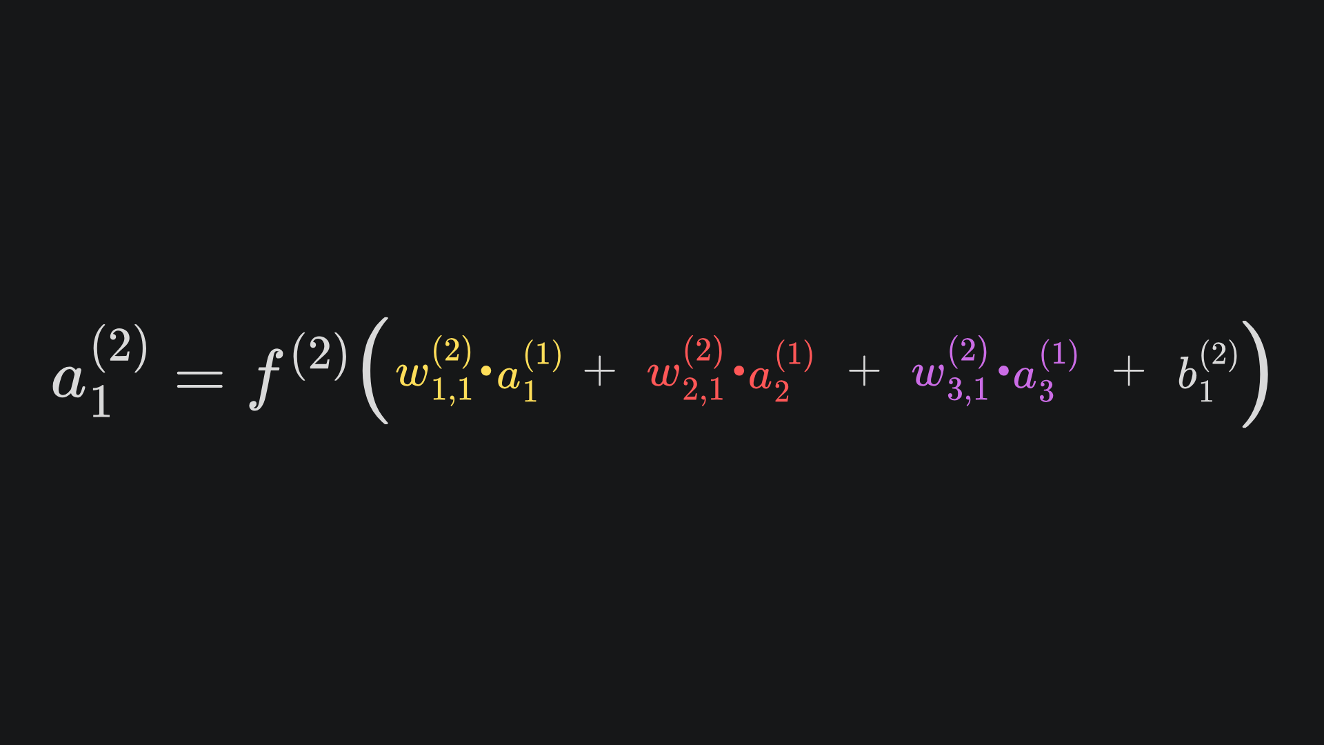
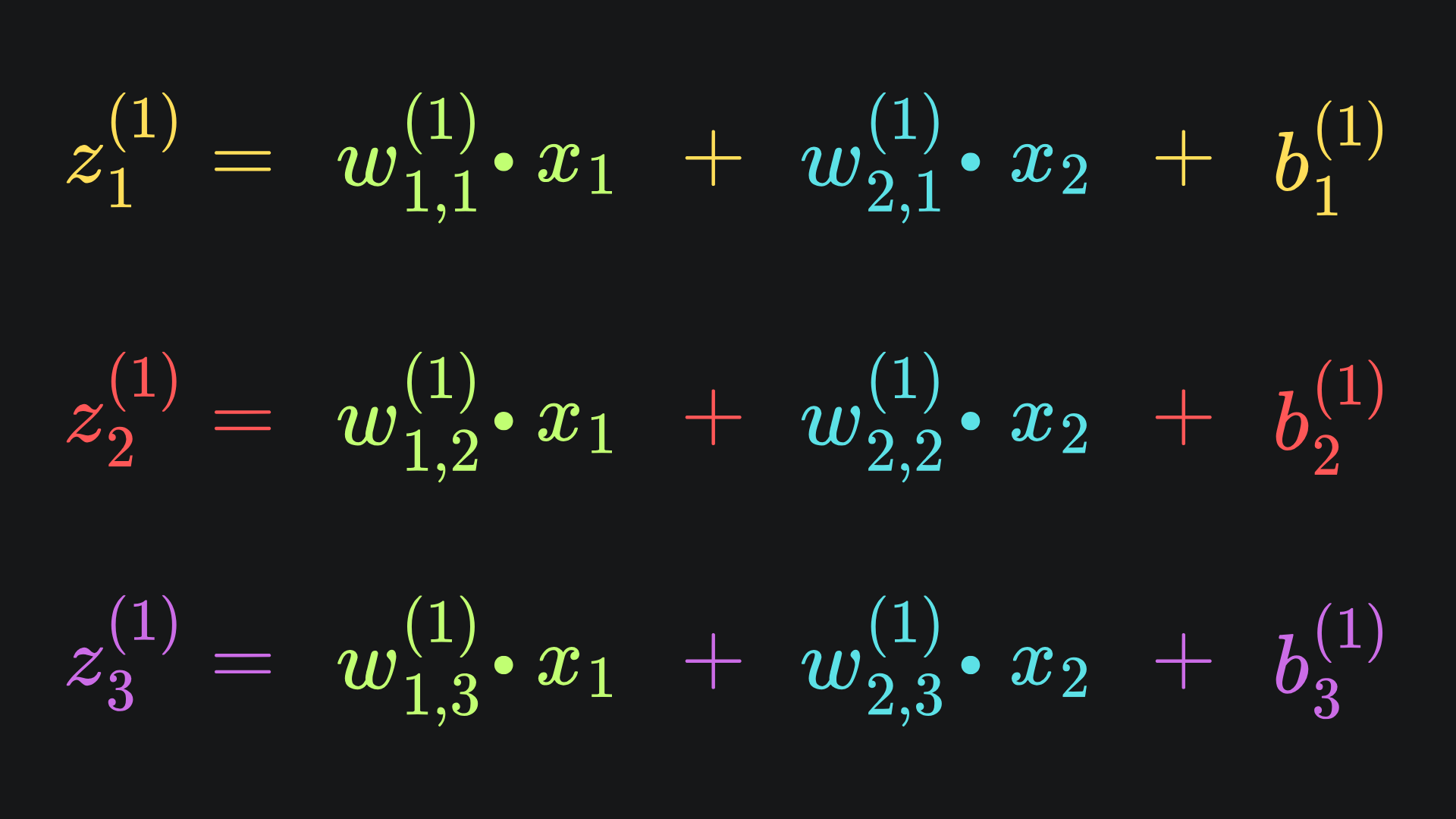
where the three input activation values can be explicitly written as

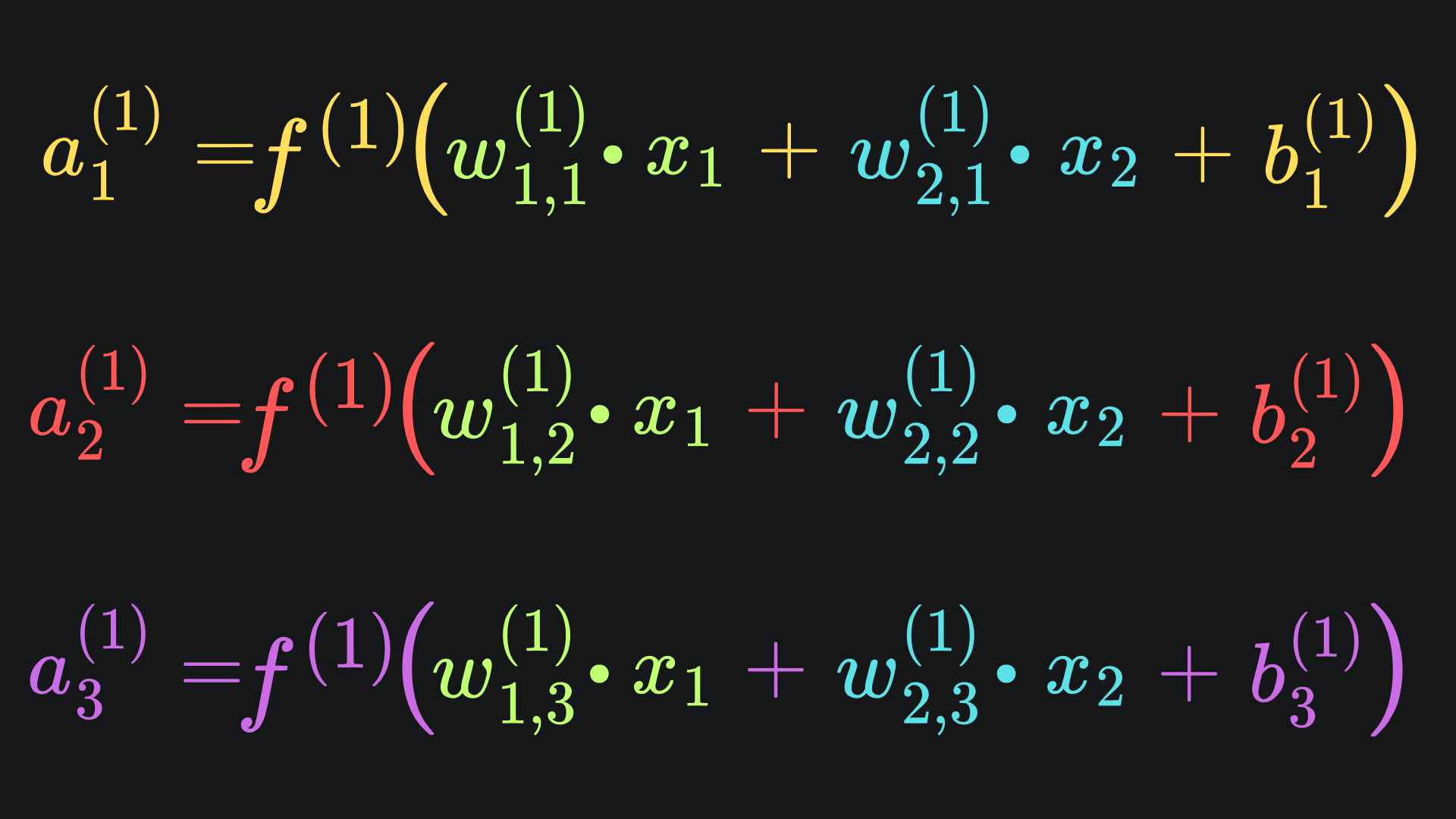
From now on, we’ll stick with just the sigmoid activation function, i.e. replace f⁽¹⁾ and f⁽²⁾ with σ.

Substituting these three expressions into the formula for a₁⁽²⁾ will give us an expression written in terms of activation functions, that are themselves expressed in terms of weights and biases. Point is, it’s weights and biases galore!

If we store all the partial derivatives of the loss function in a vector, then we can apply gradient descent on the vector’s elements. After a few iterations, we’d hope to see the loss decreasing. Here is what the vector looks like for our current example:

Vector of partial derivatives. Each element represents the partial derivative of the loss function with respect to a distinct weight/bias of the network.

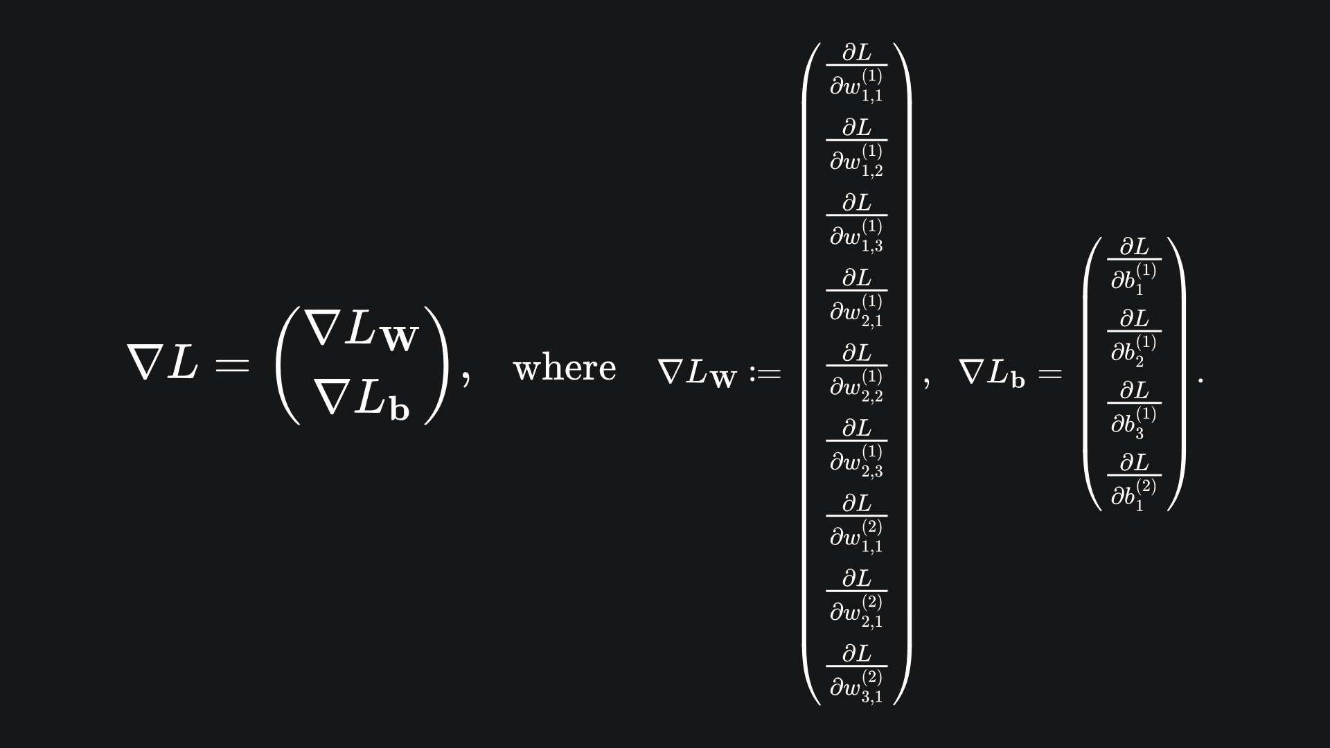
Basically, the vector ∇L has 13 elements, 9 of which are partial derivatives with respect to the network’s weights, 4 of which are partial derivatives with respect to the network’s biases. And remember, we can evaluate these explicitly, because the loss function L can be written with respect to any of these parameters, which shall be illustrated shortly.

The chain rule (again)

Each non-input node will be attributed an activation function. So the value of each output node depends on the activations from the previous layer. These activation values depend on the activations from the preceding layer, and so on until we get back to the input layer.

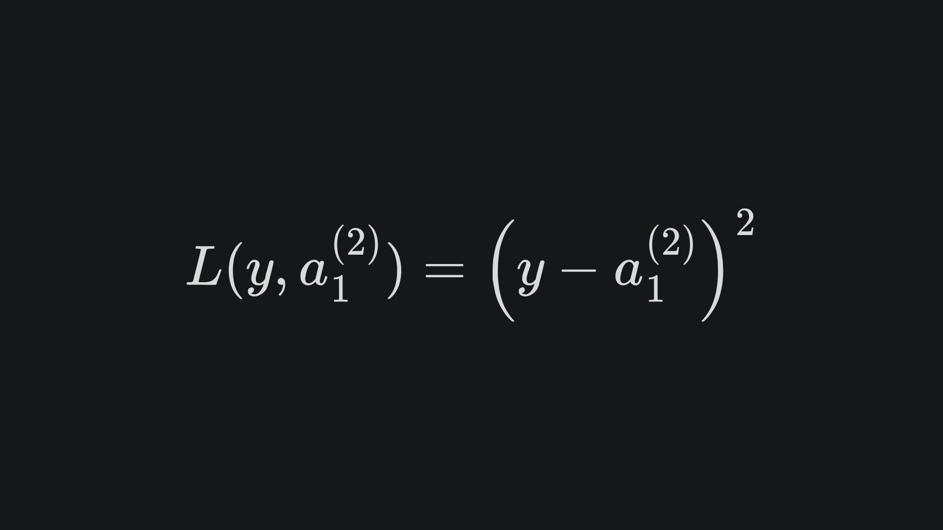
This “depends-on-the-previous-layer” idea allows us to express the loss function with respect to any weight/bias in the network. For the neural net we’ve explored so far, we can take the loss function to again be the MSE:

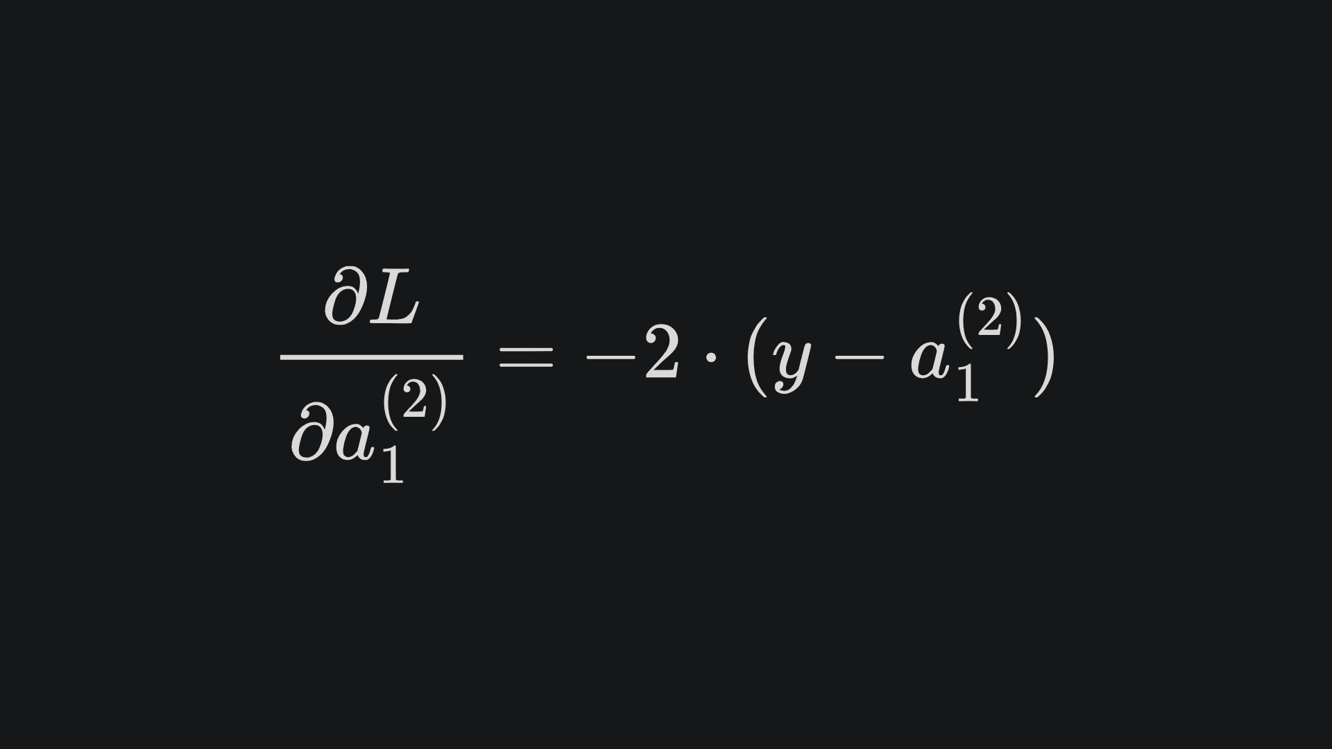
We can differentiate the loss with respect to the network prediction as in the previous example to get

Suppose that we have used the sigmoid function for all four activation functions. Then the network output is given by (follow whichever of these two is clearer to you):

At this point, we can apply the chain rule to find the partial derivative of the neural net output with respect to w_1,1⁽²⁾, w_2,1⁽²⁾, w_3,1⁽²⁾ or b₁⁽²⁾:

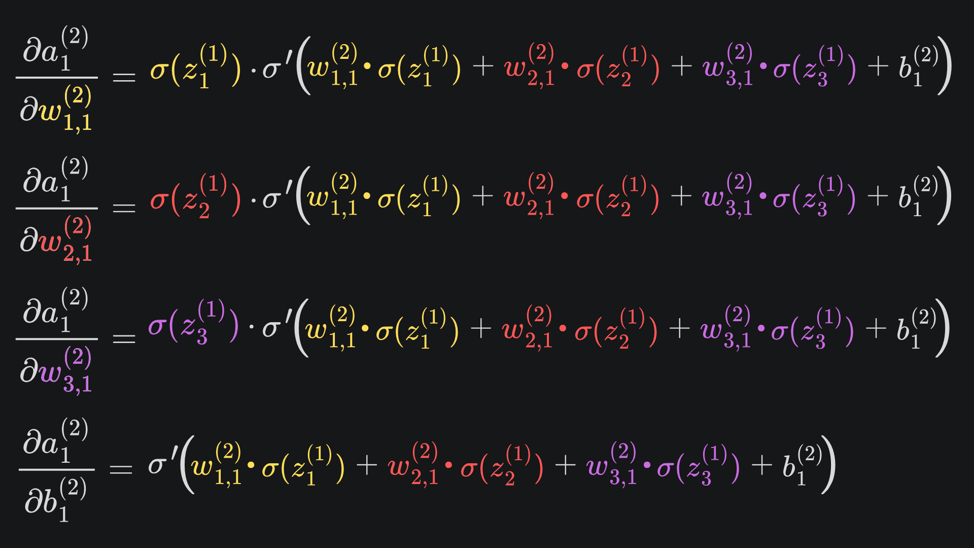
❓ Can these four expressions be evaluated ❓

Yes they can! We know what sigmoid and its derivative look like. We also know that

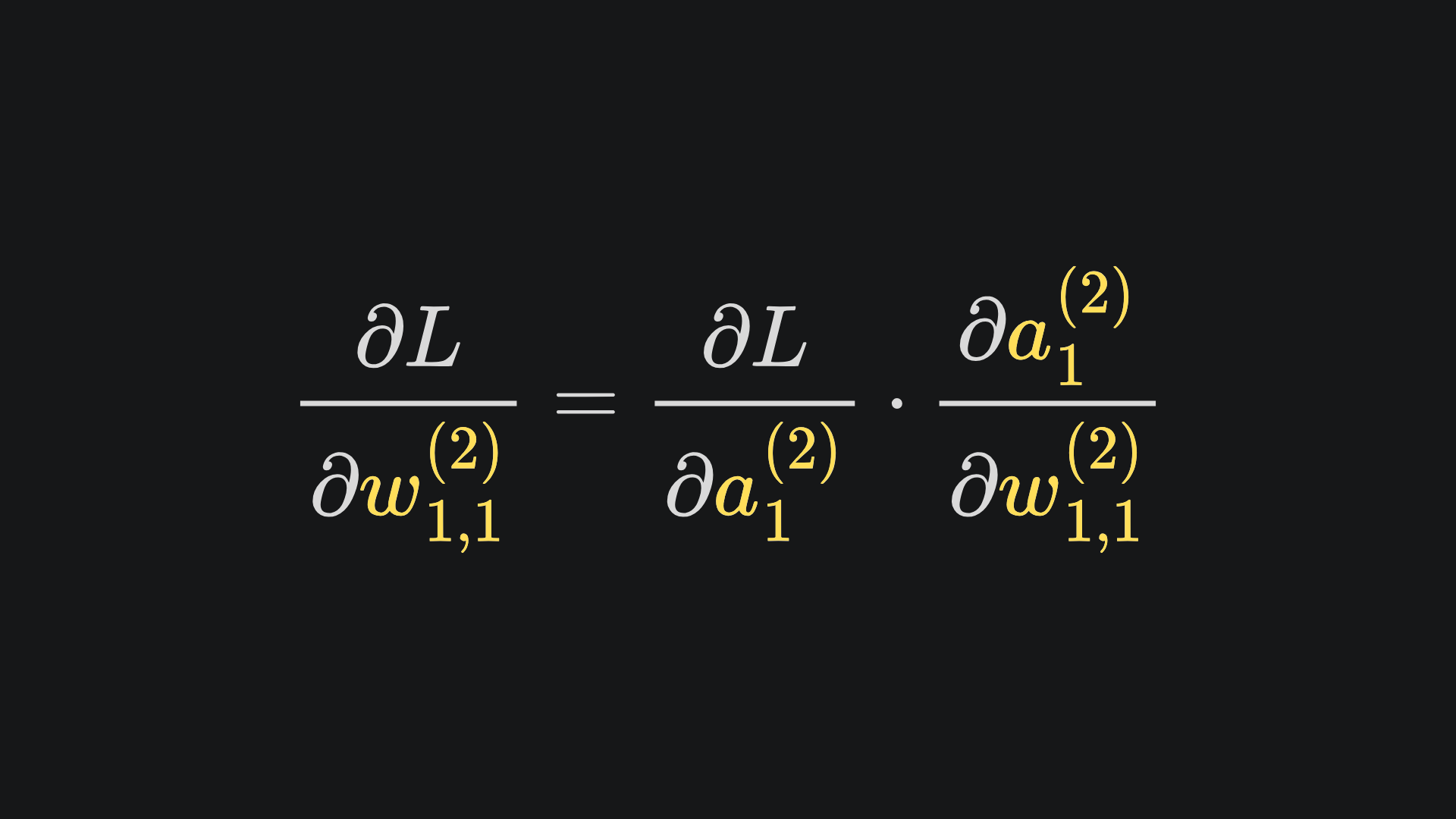
When these three are substituted into the partial derivative expressions, we’ll end up with the expressions written in terms of first-layer weights, first-layer biases and inputs x₁ and x₂. But remember that we want partial derivatives with respect to the loss function. Luckily, the chain rule saves us with

The same logic applies to the partial derivatives for w_2,1⁽²⁾, w_3,1⁽²⁾ and b₁⁽²⁾ too. Perfect 😎

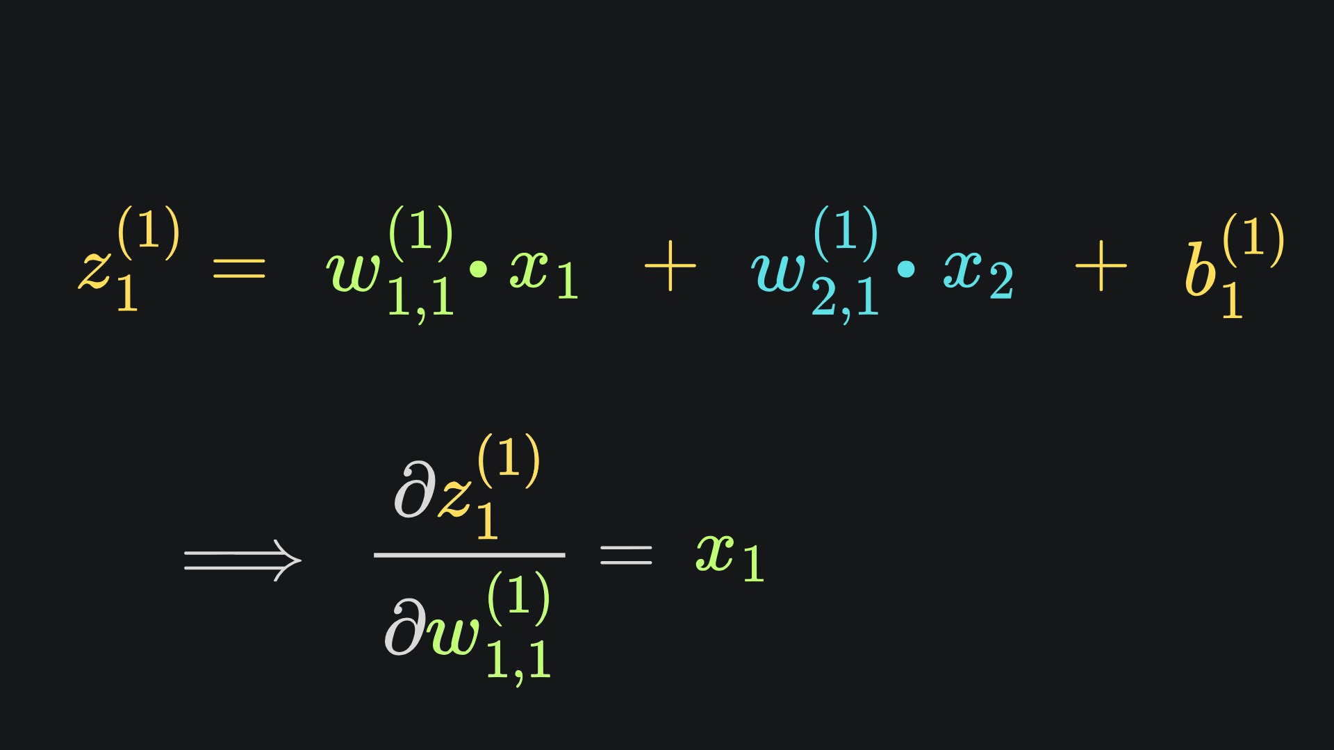
We have 9 other partial derivatives to evaluate, so it’s time to start unpacking¹ the stuff inside. Let’s start with w_1,1⁽¹⁾. We can identify the relevant dependencies from the original neural network diagram:

Observe that w_1,1⁽¹⁾ feeds into the value of z₁⁽¹⁾. The corresponding partial derivative is super easy to evaluate:

By the chain rule, we have that

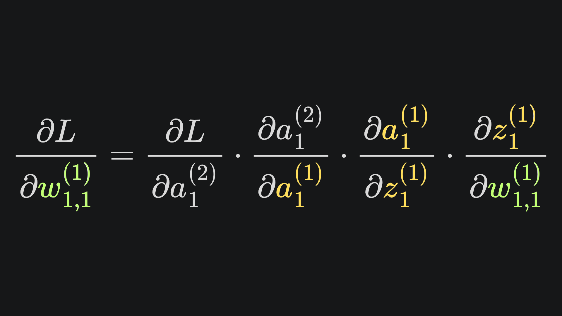
Believe it or not, we’ve already done all the heavy lifting for this. I have pasted in the four necessary partials below, mainly recapping what we’ve covered thus far:

I leave it to you to substitute in all the expressions. I’d do it myself in this article, but fear that I might get carpal tunnel syndrome if I try…

As one might imagine, the remaining 8 partial derivatives look very similar. I’d encourage you to try writing them out- the main differences will probably be what weight/bias/input you multiply the main expression by.

And just like for the initial example: (randomly) initialise the weights and biases, forward propagate to get network predictions, backpropagate, and repeat!

Packing it all up

You may have had the following insight when reading through this article: backpropagation isn’t necessarily very mathematically demanding, but rather it’s the sheer quantity of parameters and variables at play that can make it easy to lose track of what’s going on. Thankfully, we have computers to help out with all this in real life situations. And luckily for us, they’re great at all the linear algebra stuff anway. Nevertheless, I think it’s really cool to be able to understand the maths that underpins neural networks 😎

There is a non-zero chance that I have made errors in this article. Please call me out in the comments if you think I’ve slipped up anywhere!

Here’s a much-needed roundup from this time:

📦 In backpropagation, we aim to minimise the network loss with respect to the network’s weights and biases.

📦 The chain rule and partial derivatives are essential tools for understanding how backpropagation works.

📦 Backpropagation is understood best by first analysing small example networks, and then building up to larger, more complicated ones.

📦 The most complicated network we explored today had 13 parameters. But real-world neural networks? Well, the LLMs of today utilise billions of parameters. Yeah, it’s wild.

Training complete!

I hope you enjoyed reading as much as I enjoyed writing 😁

Do leave a comment if you’re unsure about anything, if you think I’ve made a mistake somewhere, or if you have a suggestion for what we should learn about next 😎

Until next Sunday,

Ameer

PS… like what you read? If so, feel free to subscribe so that you’re notified about future newsletter releases:

Sources

• My GitHub repo where you can find the code for the entire newsletter series: https://github.com/AmeerAliSaleem/machine-learning-algorithms-unpacked

1. We’re really putting the “Unpacked” in “Machine Learning Algorithms Unpacked” now, aren’t we? 🤩