Introducing non-linearity in neural networks with activation functions

Sigmoid, tanh, ReLU, LReLU, ELU and softmax.

Hello fellow machine learners,

Last week, we introduced neural networks: their architectures, parameters, and briefly described the forward passes + backpropagation that enables them to learn.

But with the way we introduced neural networks, two crucial problems were encountered:

😕 A linear combination of linear combinations is itself a linear combination. This means that, as it stands, our neural networks cannot capture non-linear patterns, which greatly restricts the circumstances in which they can be applied.

😕 Currently, our neural network outputs can take any value between −∞ and ∞. Not ideal, as this could lead to weights and biases in different layers with values that are several orders of magnitude apart, potentially inhibiting the training process.

Today, we shall resolve these issues via activation functions. These functions will introduce useful non-linearities and scaling to help us break out of linearity purgatory.

I actually have a bunch of my previous articles that I recommend you take a look at before this one. Alternatively, you can continue reading this article and refer to a few of these if you feel like you’re missing some context:

🔐 I would of course highly recommend last week’s Neural networks 101

🔐 Loss functions for classification were covered in What is the cross-entropy loss for an ML classifier?

🔐 Be sure to read Loss functions for ML regression models for, you guessed it, loss functions for regression

🔐 It could be helpful to look at the maths in Build your first linear regression model in two lines of code

🔐 We’re gonna talk about the Sigmoid activation function today, which I discussed a bit in The one equation you need in order to understand logistic regression

With all the preamble out of the way, let’s get to unpacking!

Updating last week’s architecture diagrams

If we want to introduce non-linearity to our neural networks, we have to introduce some non-linear functions. More specifically, activation functions, which are applied after taking linear combinations of weights, node values and bias values.

The diagrams that we went through in last week’s article are incomplete; they don’t factor in activation functions. Let’s fix that now, and then showcase some activation function examples after. There’s no better place to start than our main example from last time:

Neural network architecture without activation functions.

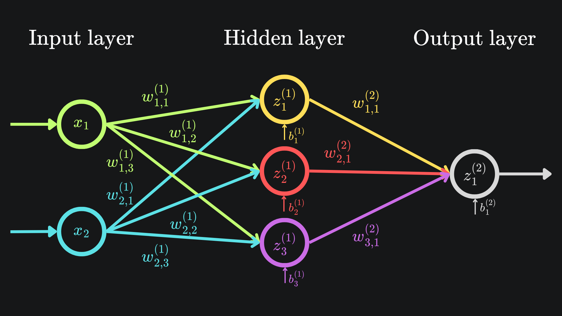
The z-values are still important, but now we apply an activation function to each non-input node before sending the value across to the next node(s) in the network:

Ahh, I see… wait, did anything even change?

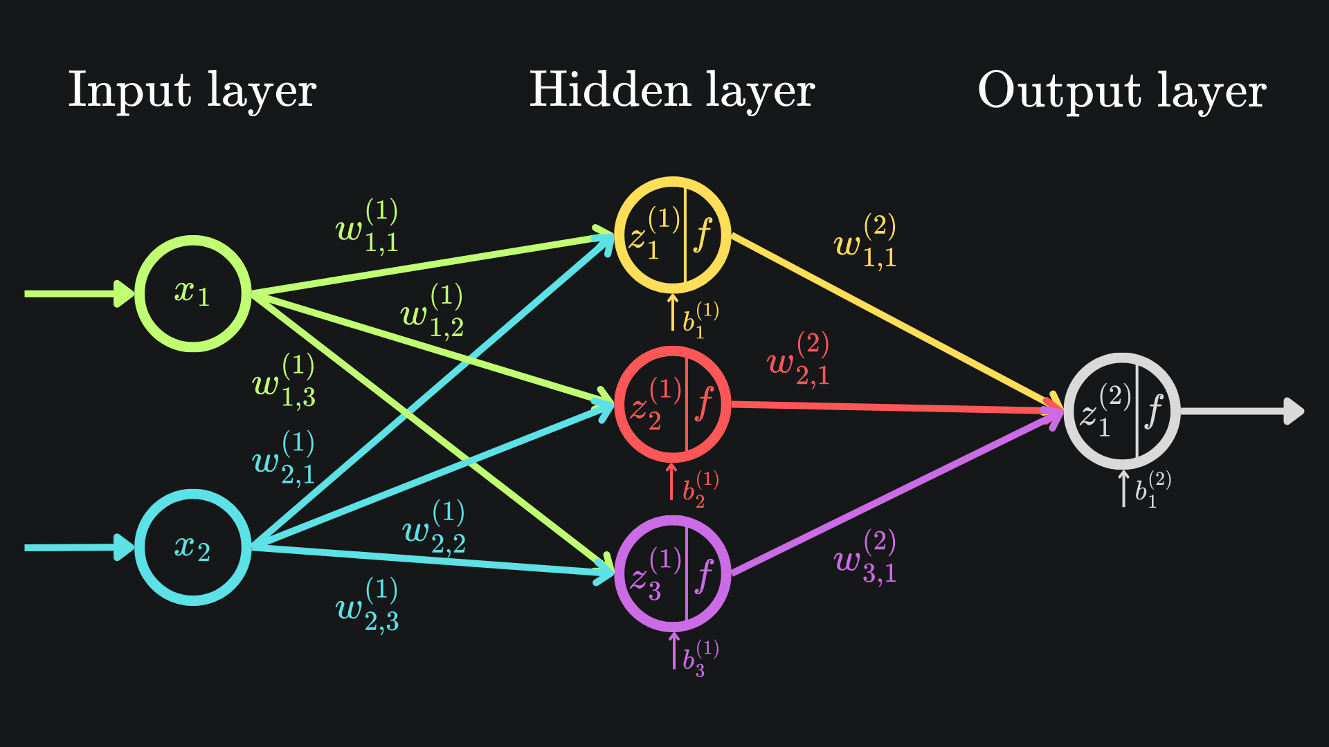
The diagram looks almost identical the first. But there’s one crucial difference. Well, technically four crucial differences. The nodes in the hidden and final layers have been modified to indicate that an activation function is being used. From now on, we will refer to the output value of a neuron as its activation value¹.

🧠 The activation a_i^(k) denotes the activation value of node i in layer k.

This means we have to update the mathematical formulas outputs of the nodes from last time. The general rule of thumb is that a_i^(k) = f(z_i^(k)), where f is the activation function of choice:

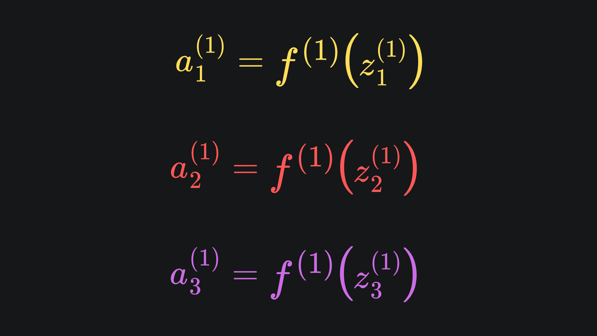
The activation functions across the entire network need not be the same, but it’s common practice to use the same activation function for all the nodes in the same layer. Hence, f⁽¹⁾ refers to the activation functions used in the first hidden layer.

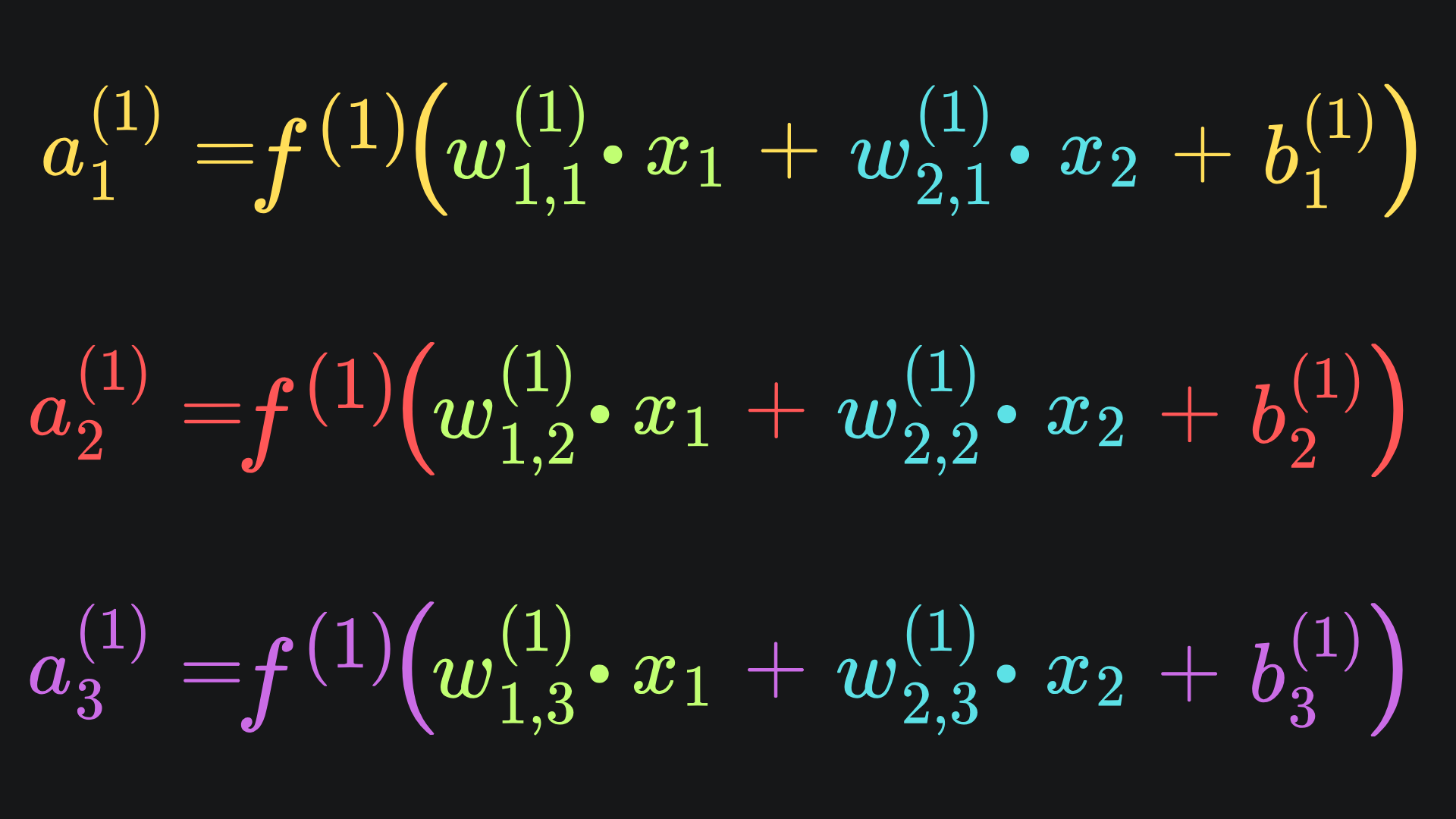
And we can write this relationship out in terms of weights, biases and inputs:

Therefore, we can update our work from last week: the final output of the neural network is now given by

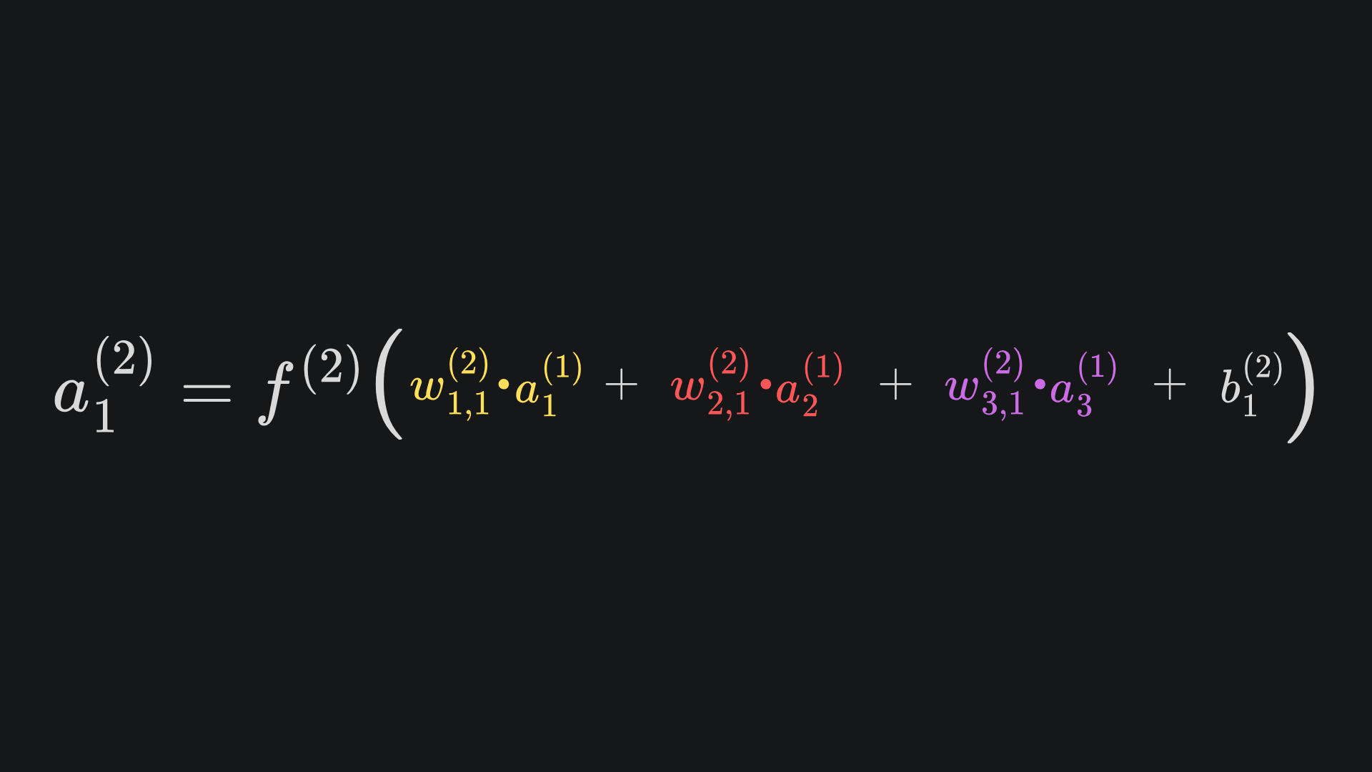
The main differences are that we have wrapped the original expression with the activation function f⁽²⁾ and have replaced z_i^(j) values with their corresponding activation values a_i^(j). But it’s what those symbols represent that’s important.

Activation functions

There are a few industrial standard examples we’ll go through in the next few subsections:

Sigmoid activation

The Sigmoid function is defined as

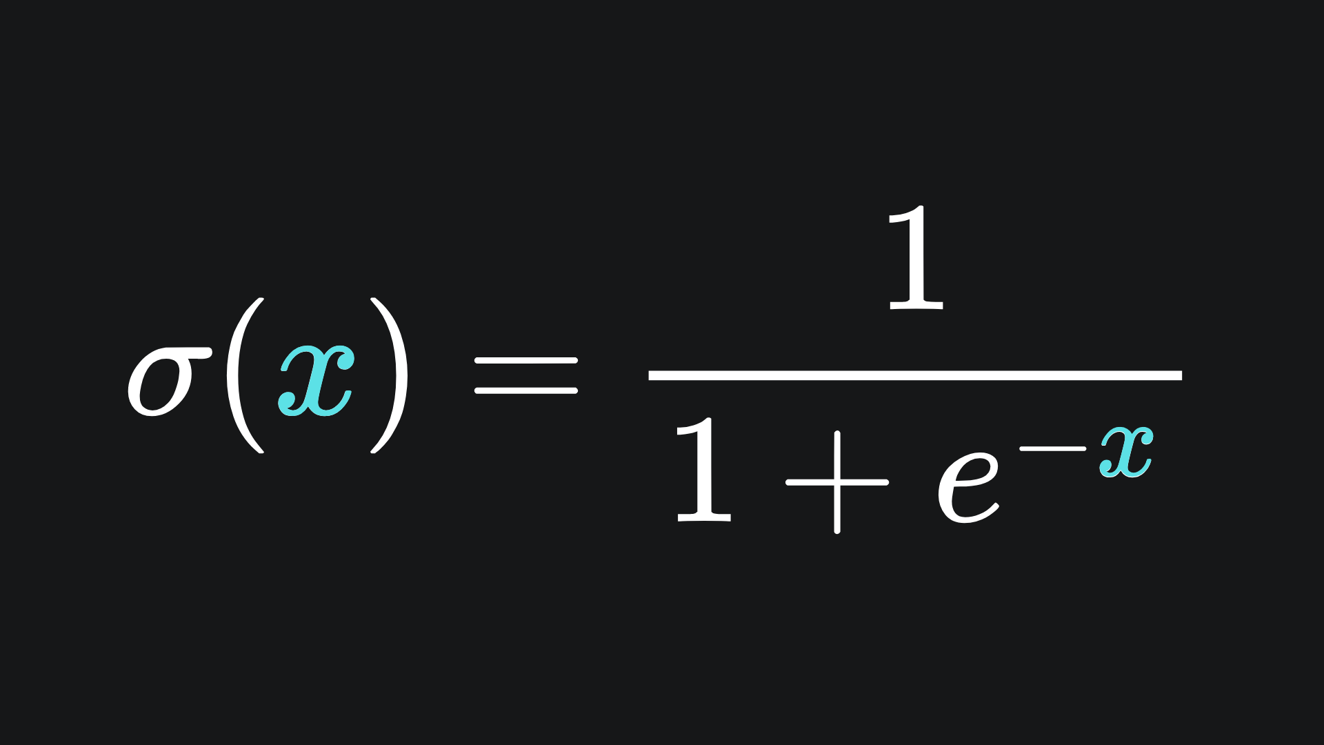
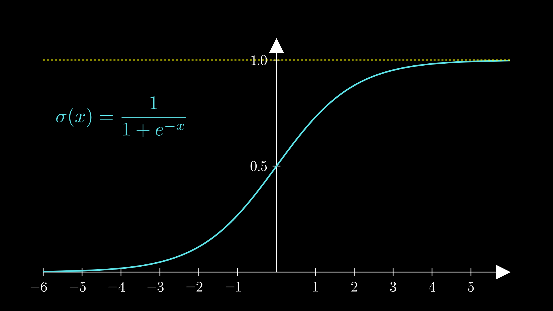
Crucially, the function takes any input and maps to the interval (0,1). Large positive values are mapped closer to 1, large negative values are mapped close to 0, and the origin is mapped to the point 0.5:

Moreover, the derivative of the sigmoid function takes a rather convenient form:

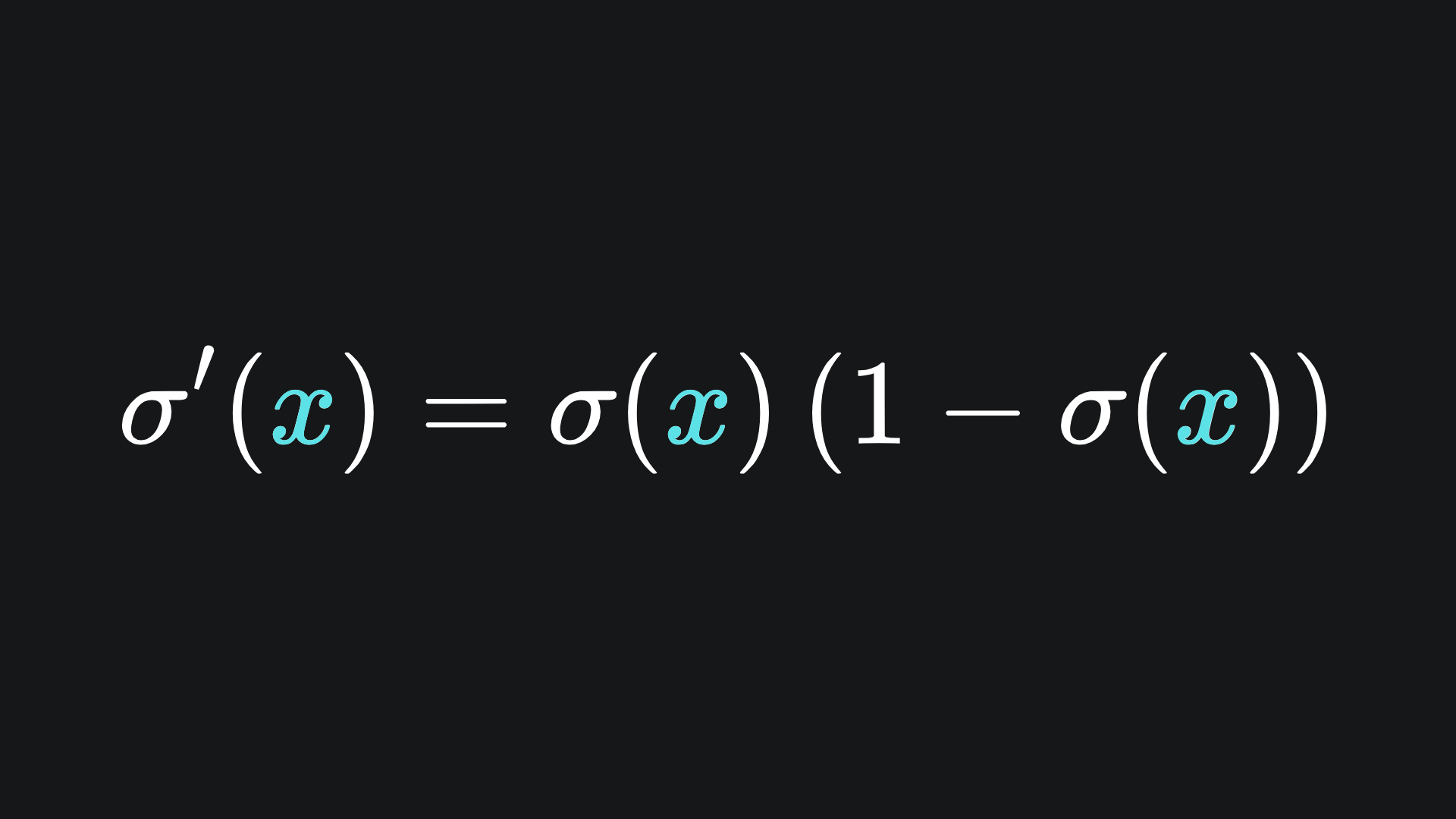
It’s a good idea to try verifying this by hand! Although the derivative takes this nice form, it can still be computationally intensive to evaluate due to the exponential function, especially if the activation is applied to many nodes of a neural network.

Tanh activation

Another common activation function is that of the tanh activation function:

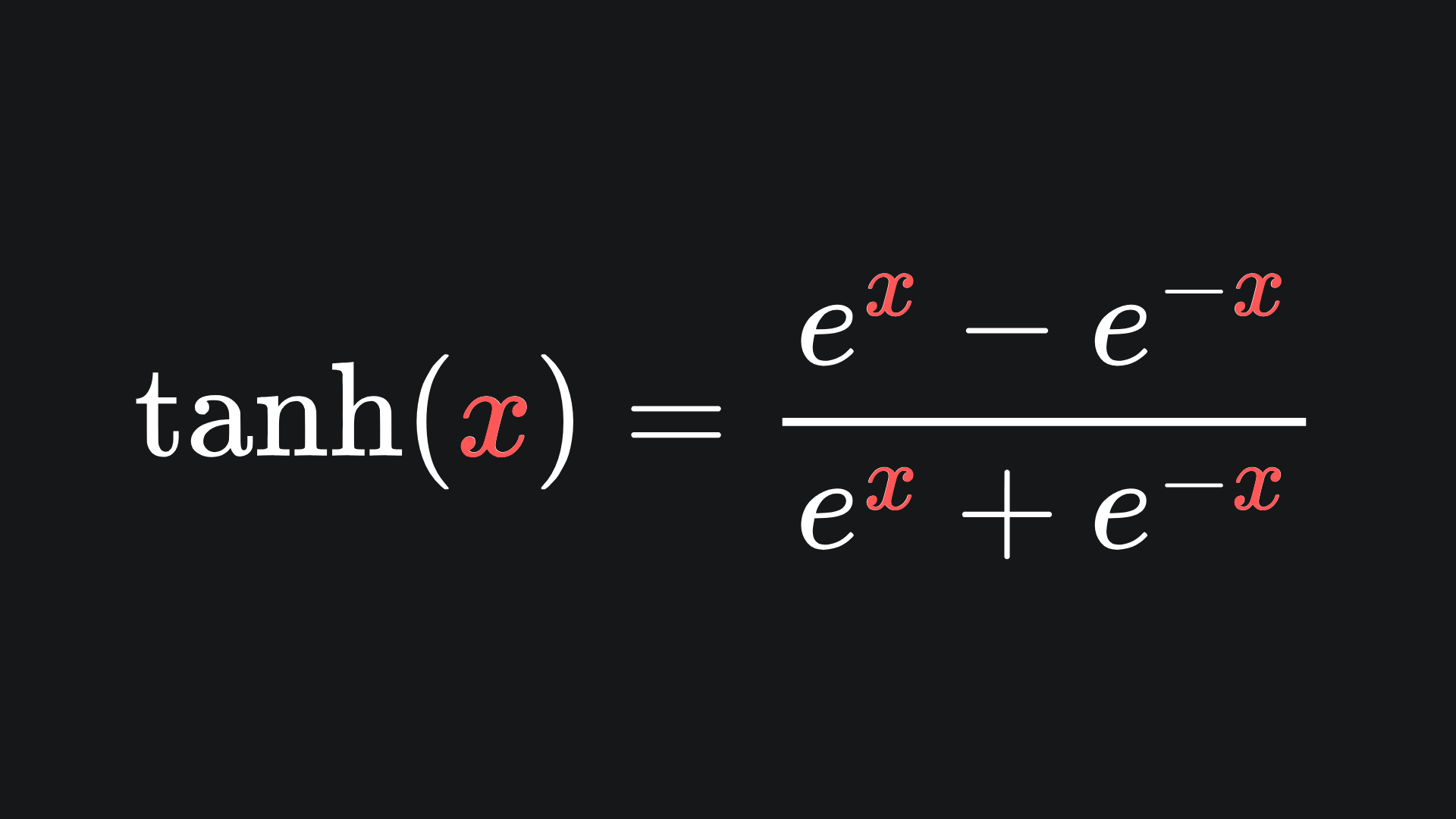
Here is the plot of the function:

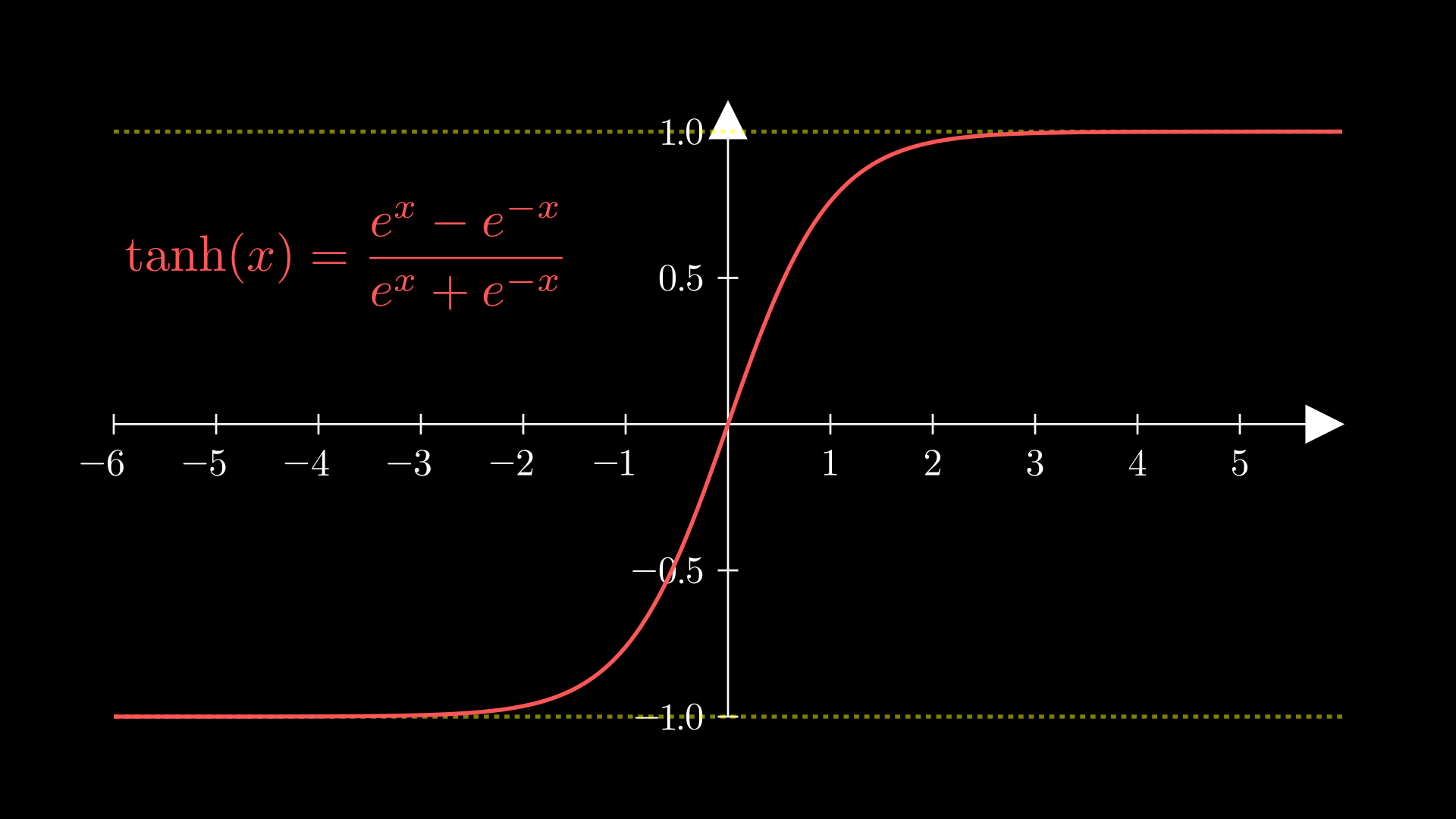
We see that tanh scales inputs down into the interval (-1,1).

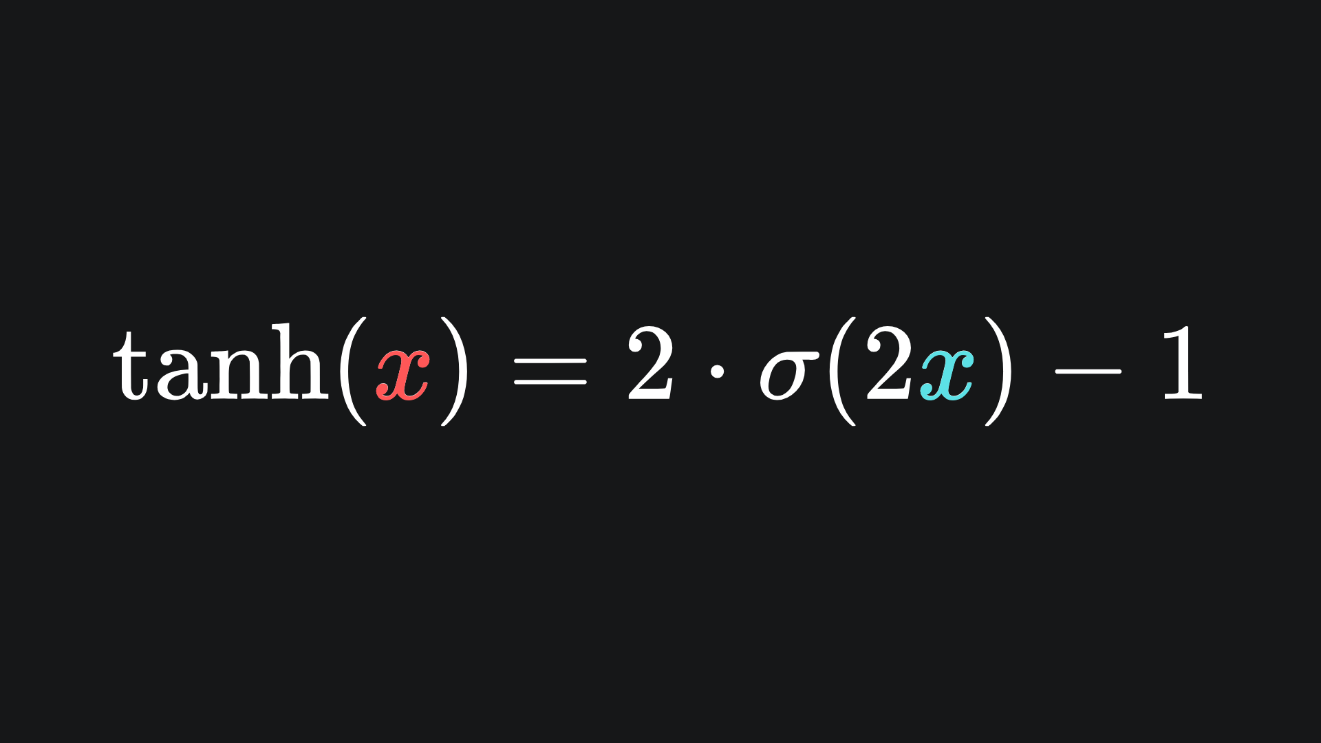
The tanh function is actually a transformation of the sigmoid function, which is another fact that you can verify for yourself:

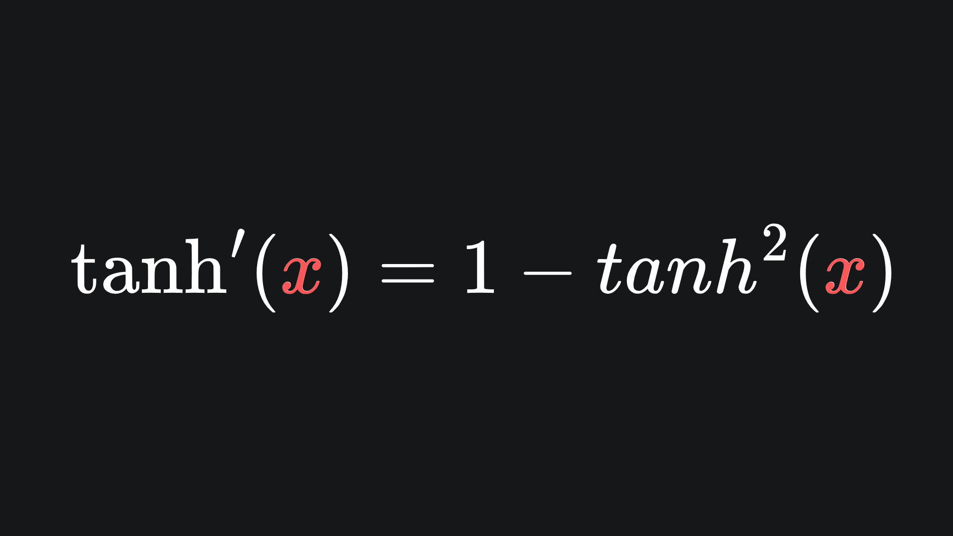
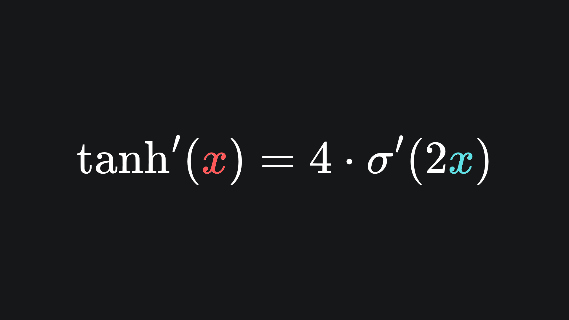
The derivative is given by

and the derivative in sigmoid form is given by

There are two main differences between sigmoid and tanh:

🧠 Tanh is centred around the origin, whereas sigmoid is not.

🧠 The gradient of tanh spikes more at 0, as shown in the below plot:

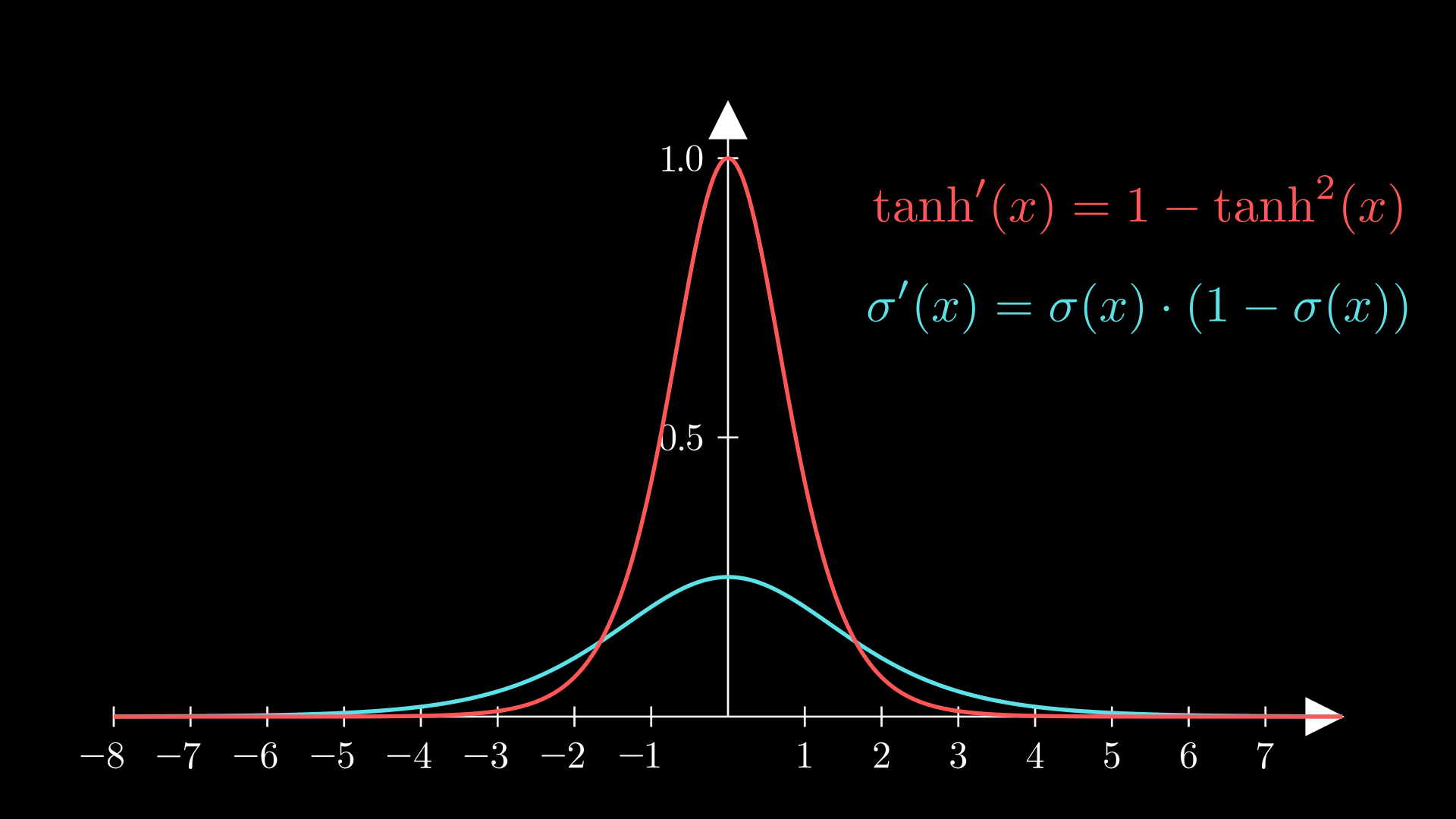
So sigmoid and tanh are great at scaling input values. However, we observe that the gradients of these functions reduce to very small values very quickly. This means that, when implementing gradient descent, weight and bias values may not change much between iterations. This is called the ‘vanishing gradient problem’.

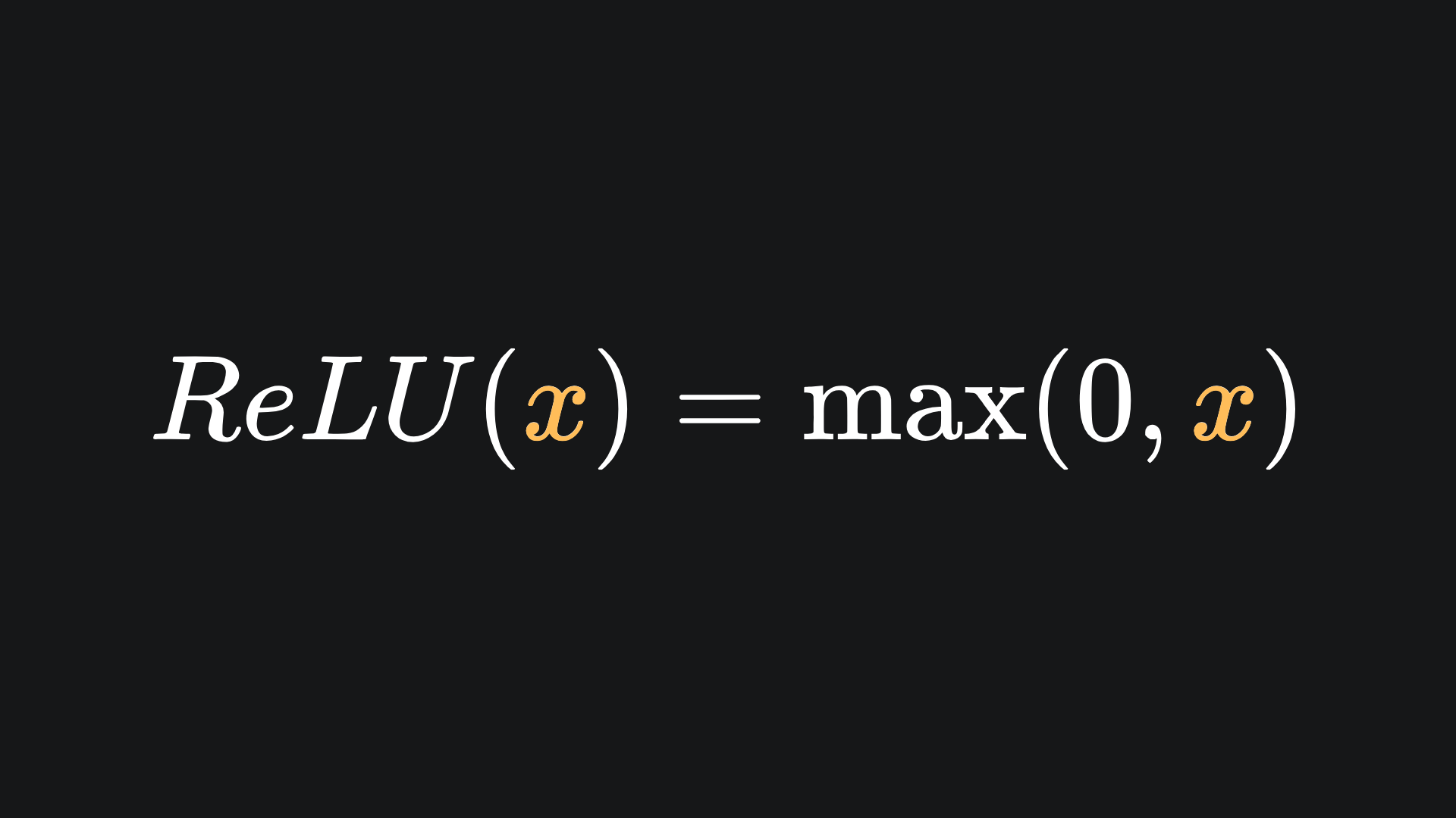
ReLU activation

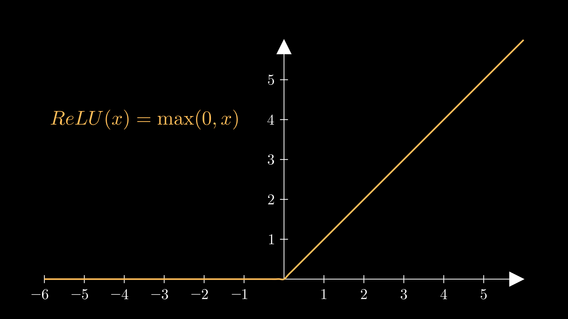
The vanishing gradient problem of sigmoid and tanh can be partially resolved with the ReLU function. ReLU, which stands for Rectified Linear Unit, is almost the same as the identity function, except it evaluates to 0 for negative inputs:

This is what it looks like:

The formula for the derivative of ReLU, as well as the graph of the derivative, are shown below:

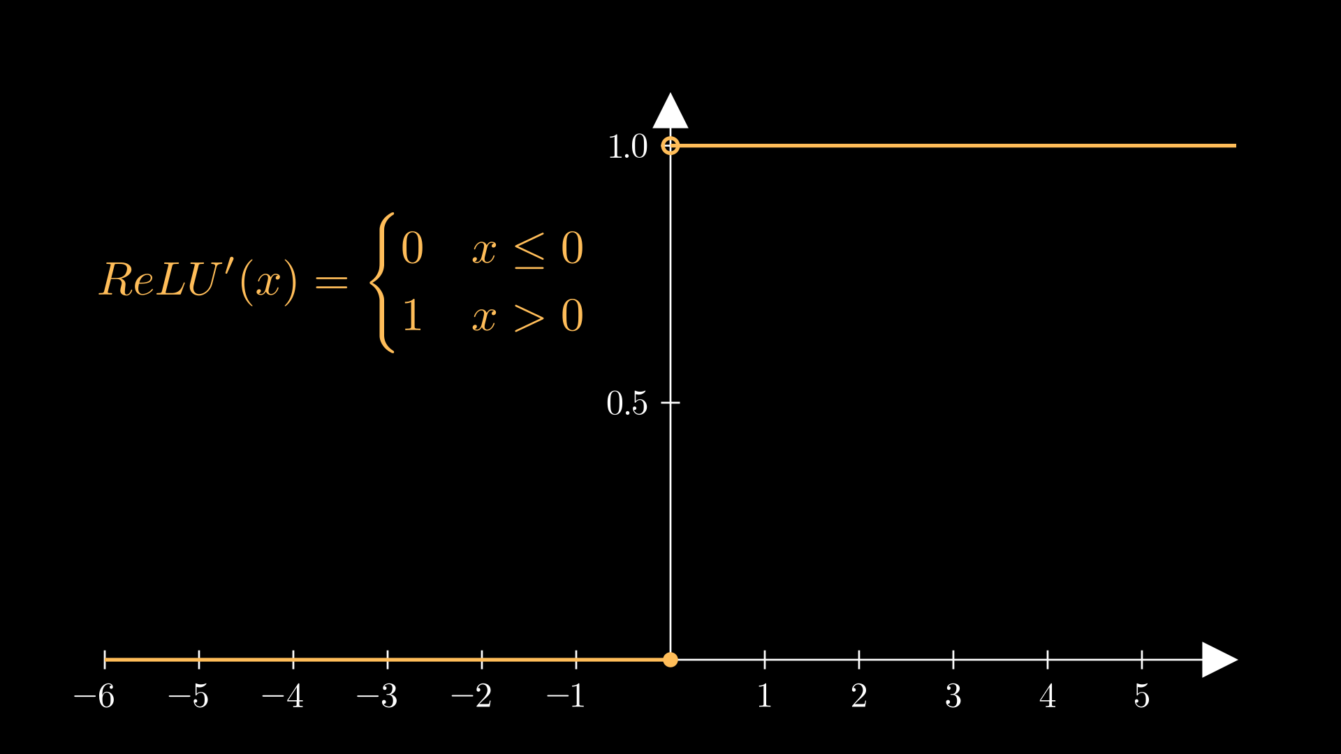
Uh oh- we seem to have a problem at x=0. It turns out that ReLU isn’t differentiable at 0 thanks to the kink at the function’s origin. For a mathematician like me, this is enought to send one into panic mode. But in practical ML code packages, the gradient at 0 is just set to just be be either 0, 0.5 or 1.

Moreover, while the gradient of ReLU is just 1 for positive inputs, it goes to 0 for negative inputs. This is in stark contrast to sigmoid and tanh: where they suffer from the vanishing gradient problem, ReLU has precisely zero gradient for negative values. However, sigmoid and tanh suffer their gradient issues for both positive and negative values, whereas with ReLU, positive inputs won’t suffer these problems. As such, gradient descent for positive ReLU will flow fine, but once an input goes negative, the corresponding node’s value stays stuck at 0, no matter what gradient descent procedure is used. This is called the ‘dead ReLU problem’.

Leaky ReLU activation

One way to solve the dead ReLU problem is to add a non-horizontal gradient to the left side, parametrised by a small positive parameter α. The formula for the Leaky Rectified Linear Unit (abbreviated to LReLU) is

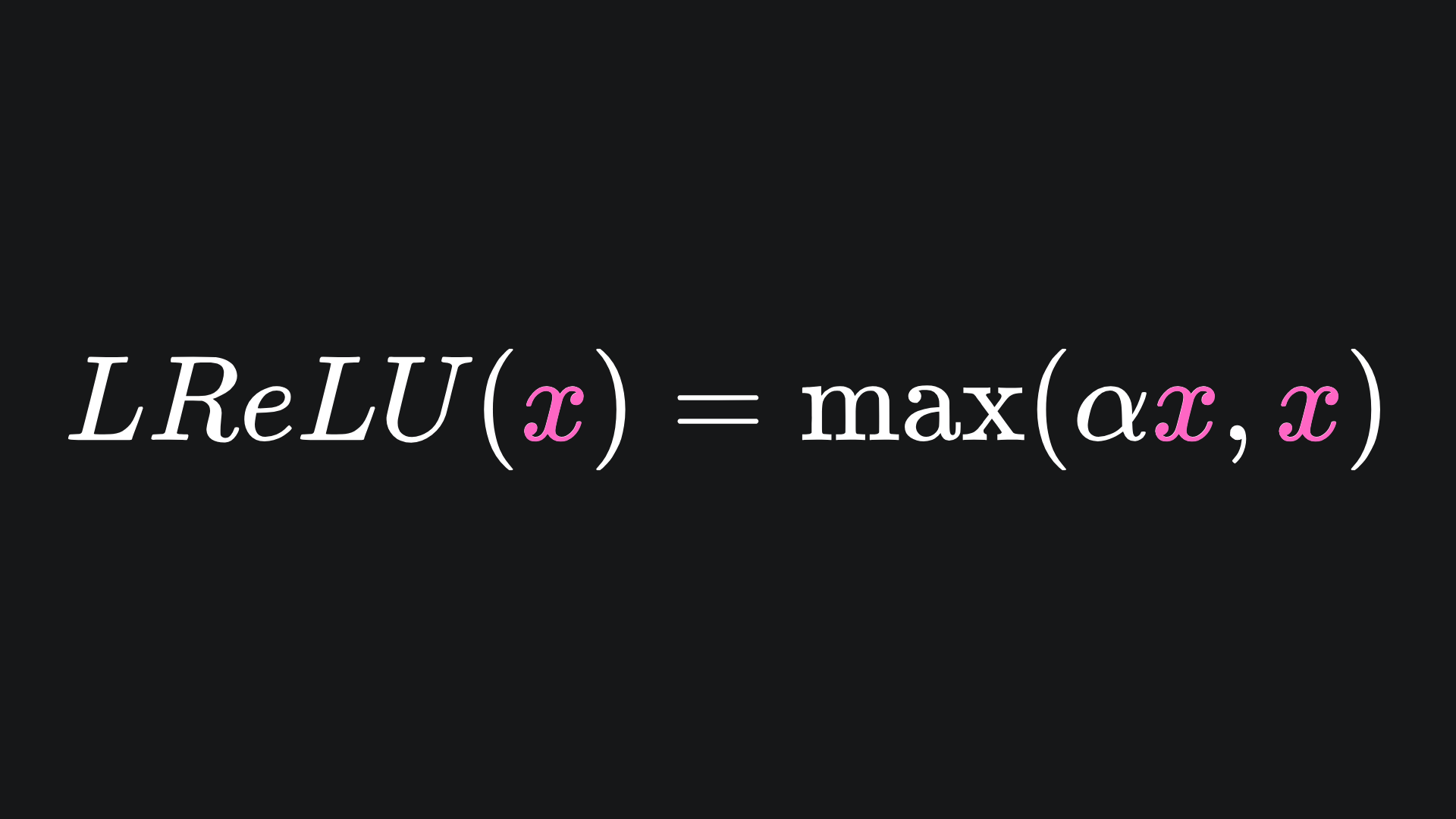
and the function is shown below:

The default value for α in PyTorch is 0.01, but this can be experimented with in practice. The ‘leaky’ part of LReLU helps us escape from the dead ReLU issue we had before.

The gradient for LReLU is as you’d expect:

Although we have a nice continuous derivative when α=1, it doesn’t make sense for us to use this value in practice, because then we just end up with the identity activation function f(x)=x.

Exponential Linear Unit (ELU) activation

Another solution to the dying ReLU problem involves the use of an exponential component for negative inputs:

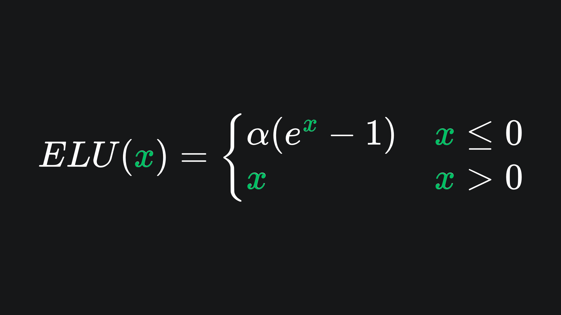
As usual, let’s explore both what the function looks like:

as well as its gradient function:

This activation function solves the dying ReLU problem outright, with non-zero gradient for negative inputs that aren’t too far below 0. What’s more, setting α=1 (the default value in PyTorch) helps to fix the differentiability problem at x=0! However, the price you pay is a computational one, as the value of the exponential must be computed each time you want to apply the activation.

Softmax activation

Let’s wrap up with an activation function for an entirely different use case.

Suppose that you want your neural network to make a prediction from one of n categories. For example, in a sentiment analysis task, you might pass text data into the network and ask it to predict whether the input text is positive, negative or neutral in sentiment.

How would we configure the output layer of a neural network for this classification task?

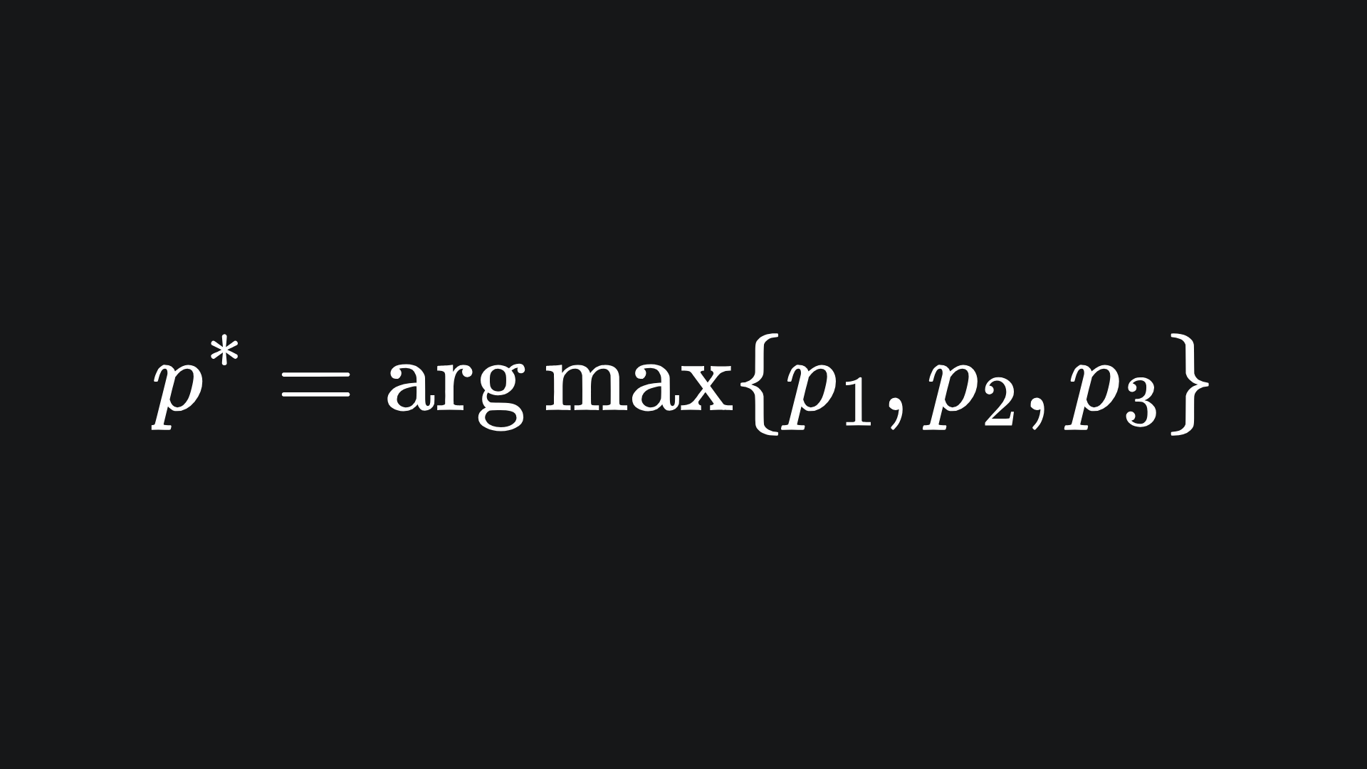
The solution is as follows: treat the values in the output layer as probabilities. In the context of our sentiment analysis task, we treat the three outputs as p₁, p₂ and p₃ and assert that p₁+p₂+p₃=1. We then assume the network output to be the probability index with the largest value:

In order to map the network’s computations to probability values, we use the softmax function. For the input vector x={x₁, x₂,…, x_n}, The i-th probability value p_i is given by

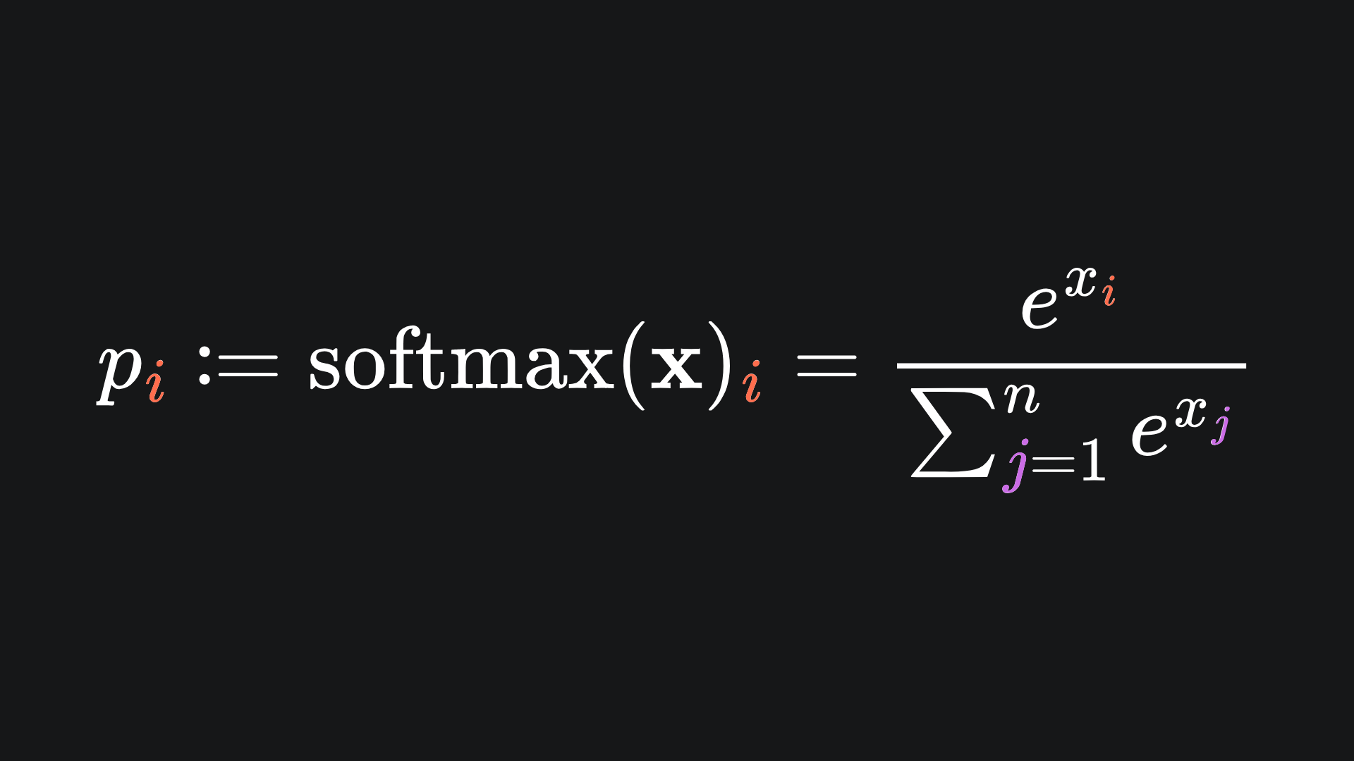
The exponential function ensures that all inputs get mapped to a positive value.

It’s actually pretty easy to verify that our claimed ‘probability values’ sum to 1 as they ought to:

In the penultimate line, the numerator and denominator are in fact equal, hence the fraction simplifies to 1.

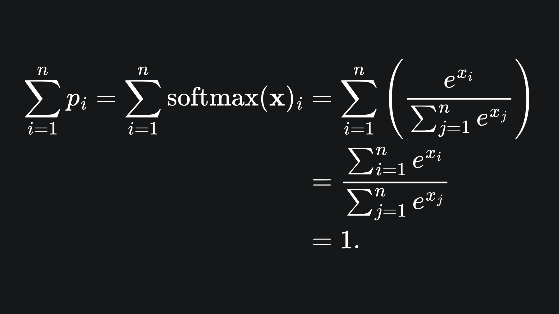
Each probability can be thought of as the confidence that the model has in that category of classification. So if the values were 0.15, 0.80 and 0.05 for positive, negative and neutral sentiments respectively, then we can think of the model as having 80% confidence that the input text is negative in sentiment.

Packing it all up

Phew, plenty of functions discussed in this one! When building your own neural networks with a Python package like PyTorch or TensorFlow, you can specify what activation functions you want to be used in each layer. And you hopefully now have a better understanding of what these activations actually do. Nice!

Now for your weekly roundup:

📦 The sigmoid and tanh functions are s-shaped curves that scale input values to a manageable range. However, they suffer the issue whereby the gradient ‘vanishes’ for input values that are large in magnitude, which hinders algorithms like gradient decent from doing their job well. Additionally, these functions are computationally demanding to evaluate, especially for neural nets that have lots of layers and parameters.

📦 The Rectified Linear Unit (ReLU) has good gradient flow for positive input values, but in fact suffers from the ‘dying ReLU problem’ for negative inputs. That said, it’s super easy to evaluate the ReLU function compared to sigmoid and tanh.

📦 LReLU and ELU take different approaches to solve the dying ReLU problem, but in both cases you’ll need to play around with the α parameter for the best results.

📦 The softmax activation function can be used in the output layer of a neural network that’s designed for classification tasks.

Training complete!

I hope you enjoyed reading as much as I enjoyed writing 😁

Do leave a comment if you’re unsure about anything, if you think I’ve made a mistake somewhere, or if you have a suggestion for what we should learn about next 😎

Until next Sunday,

Ameer

PS… like what you read? If so, feel free to subscribe so that you’re notified about future newsletter releases:

Sources

• My GitHub repo where you can find the code for the entire newsletter series: https://github.com/AmeerAliSaleem/machine-learning-algorithms-unpacked

1. I talked mainly about ‘z-values’ thing last week, because I didn’t want to rush the discussion of activation functions, and figured that the topic deserved its own article.