
Why random forests outperform decision trees: 'bagging' for variance reduction
Explaining how the bootstrap aggregation procedure reduces the variance of an ensemble, and how the random forest extends the bagging framework.

Hello fellow machine learners,
We have spent the past few weeks discussing the decision tree algorithm. We have discussed the pros and cons of the model and are now in a good position to discuss how the predictions of multiple decision trees can be combined to produce a new, more powerful predictor.
Let’s get to unpacking!
What’s better than one decision tree?
Our aim in this article is reduce the high-variance problem of the decision tree. To do this, we will take the predictions made by a group of decision trees and take a ‘majority vote’ to classify any new data point. The process is comprised of two main steps:
For each tree, we take a sample of data rows with replacement, a process known as bootstrap sampling. We train each tree on a distinct bootstrap sample. By sampling with replacement, we allow for different training sets for each tree.
Once we have grown all the trees we want, we observe how each tree classifies the test data. The prediction made by the group of decision trees is done via aggregation, i.e. we take a majority vote from the labels assigned to the data by each tree.
In academia and industry, we shorten the ‘bootstrap aggregation’ name to just ‘bagging’. The bagging process is especially effective for low-bias1, high-variance models such as the decision tree.
Variance of an ensemble of trees
Let’s appeal to some statistics to figure out why bagging is so useful.
Suppose that we grow n decision trees in our ensemble: T_1, T_2,…, T_n. Since each tree is grown using the same recursive binary splitting procedure, the trees are identically distributed. Therefore, we can consider T_1,…,T_n as identically distributed random variables, each with, say, mean μ and variance σ^2.
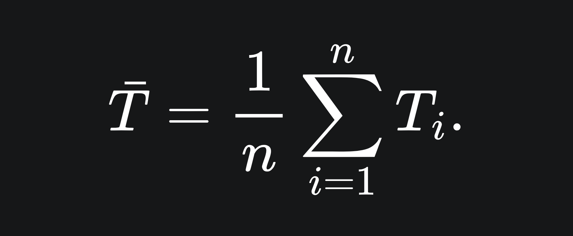
We can consider the output of the bagging procedure as the sample mean of the input trees:
The average value of the sample mean is:
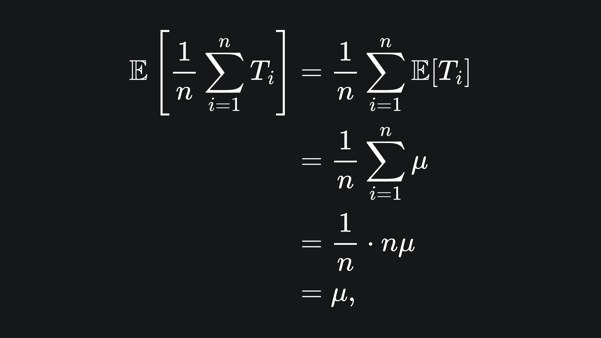
i.e. it’s the same as the mean of any tree in the ensemble.
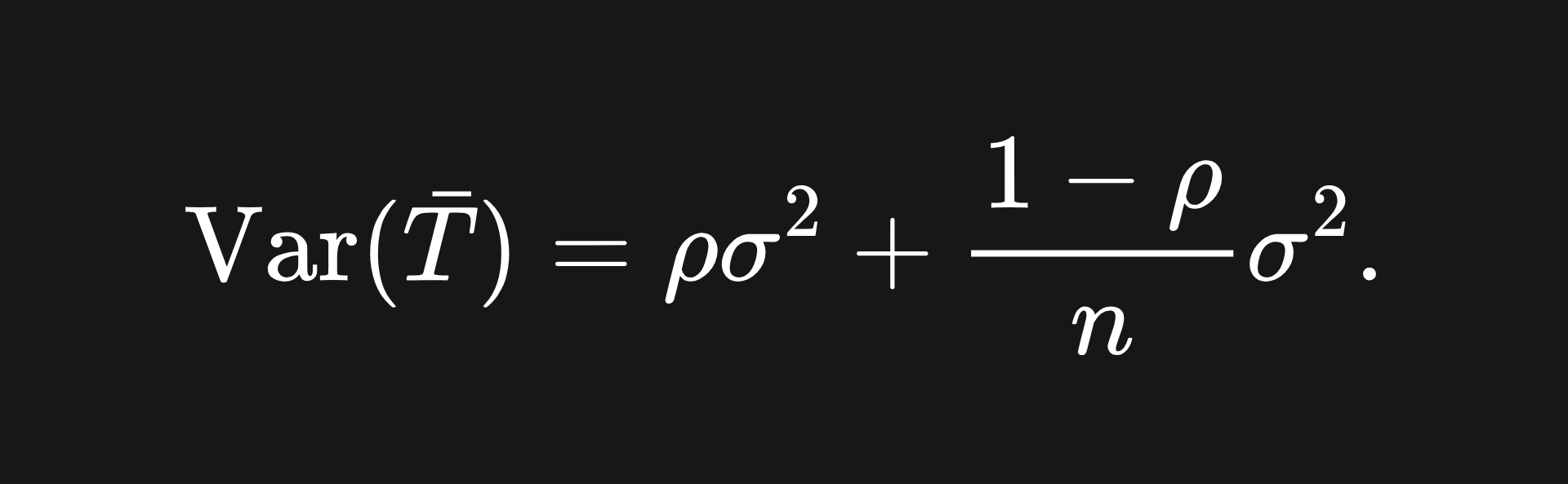
Now for the variance of the sample mean. I claim that this is given by
[Check out the Appedix section at the end of this article for the derivation.]
Notice that, for large values of n (i.e. adding more trees to the ensemble), the value of the second term is reduced. However, if our trees are correlated, then the value ρ increases, which increases the first term.
Random forest: de-correlated trees
From the previous section, we know that including more trees in our ensemble will help to reduce the variance. However, this effect will be diminished if our trees are correlated.
As well as bootstrap sampling, another thing we can do is consider only a subset of the feature space for each split. This process helps to de-correlate the trees we grow. A decision tree ensemble that utilises this technique is called a random forest.
The smaller the subset size, the less correlated the trees will be. That said, if your feature subset is too small, then you will limit the performance of that particular tree, meaning the model won’t work as well.
Random forest hyperparameters
The scikit-learn implementation of the random forest classifier has loadddddsssss of hyperparameters. Some of these relate to the individual trees grown as part of the ensemble, which we discussed last week. Here are some new ones that are relevant to our current discussion:
How many trees should we grow? [
n_estimators]Essentially, the more trees you include in your ensemble, the better the ensemble ought to perform, at the expense of computational complexity.
How many bootstrap samples should we use for each tree? [
max_samples]If the original dataset contains n rows, then we should use n rows in each bootstrap sample. Don’t forget that bootstrap sampling occurs with replacement, so we don’t have to worry about running out of data to sample.
What size of feature subset should we consider for each split? [
max_features]I have seen conflicting information about this from my reading. It is claimed in “The Elements of Statistical Learning” that the inventors of the random forest recommend a feature subset with the size of the square root of m, where m is the total number of features. This is also the default value for the scikit-learn implementation of the random forest classifier. However, in Breiman’s 2001 paper on random forests, he shows empirical results from experimentation with the feature subset size, which don’t align exactly with this claim. Thus, I would recommend that you can start with the default value of sqrt(m), but then fine-tune this hyperparameter along with the others.
Packing it all up
The random forest is one of the most commonly used algorithms in industry. And now you know the main theory behind it! We will discuss the pros and cons of the random forest after diving into another tree-based algorithm (next Sunday!).
Here’s a brief recap of everything from today:
The bagging procedure involves taking bootstrapped samples (i.e. sampling with replacement) of the training data and aggregating the predictions made on it across multiple learners.
The random forest algorithm is an extension of bagging, where the base learners are decision trees and a subset of the feature space is taken into consideration for the splitting conducted at each node.
The greater the size of the feature subset, the more powerful the corresponding decision trees, but the more correlated they will become. The aim of the random forest is to reduce variance, so one must experiment with the feature subset size to strike a good balance.
Training complete!
I hope you enjoyed reading as much as I enjoyed writing 😁
Do leave a comment if you’re unsure about anything, if you think I’ve made a mistake somewhere, or if you have a suggestion for what we should learn about next 😎
Until next Sunday,
Ameer
PS… like what you read? If so, feel free to subscribe so that you’re notified about future newsletter releases:
Sources
“The Elements of Statistical Learning”, by Trevor Hastie, Robert Tibshirani, Jerome Friedman: https://link.springer.com/book/10.1007/978-0-387-84858-7
“Random Forests“, by Leo Breiman: https://link.springer.com/article/10.1023/A:1010933404324
The scikit-learn implementation of the random forest classifier: https://scikit-learn.org/stable/modules/generated/sklearn.ensemble.RandomForestClassifier.html
Appendix
In this section, we verify the formula for the variance of the sample mean T̅. We mainly follow the solution for Exercise 15.1 of “The Elements of Statistical Learning”.
Since the T_i are not necessarily independent, we cannot ignore the covariances. The (product moment) correlation coefficient between any T_i and T_j is given by
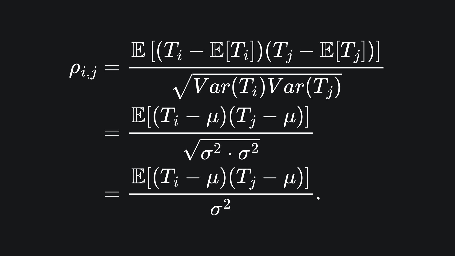
Expanding out the numerator and rearranging yields
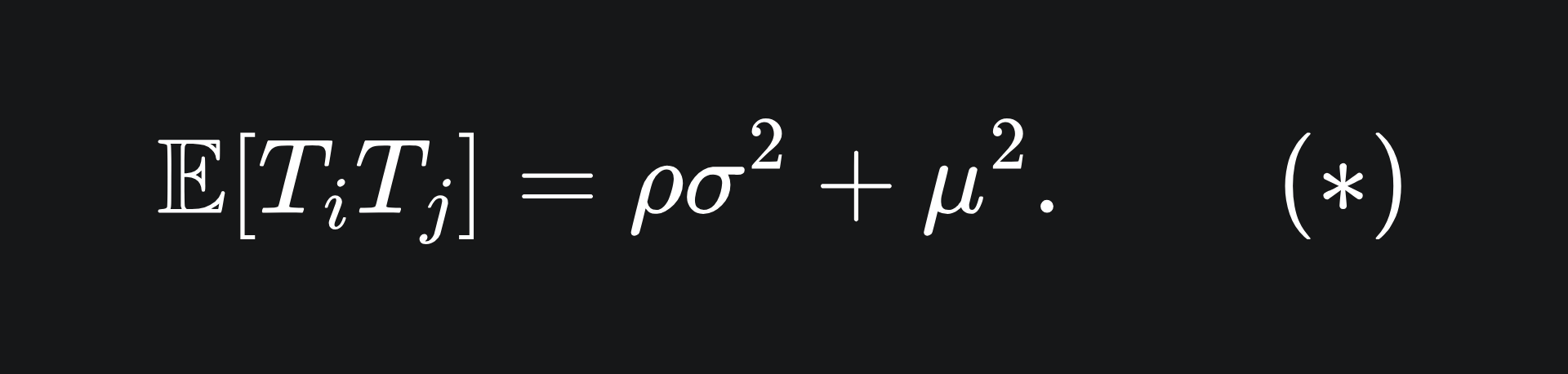
As the T_i and T_j are identically distributed, we can drop the subscript on ρ. But note that ρ=1 if i=j, a fact we will use later.
Now, the variance of the sample mean is
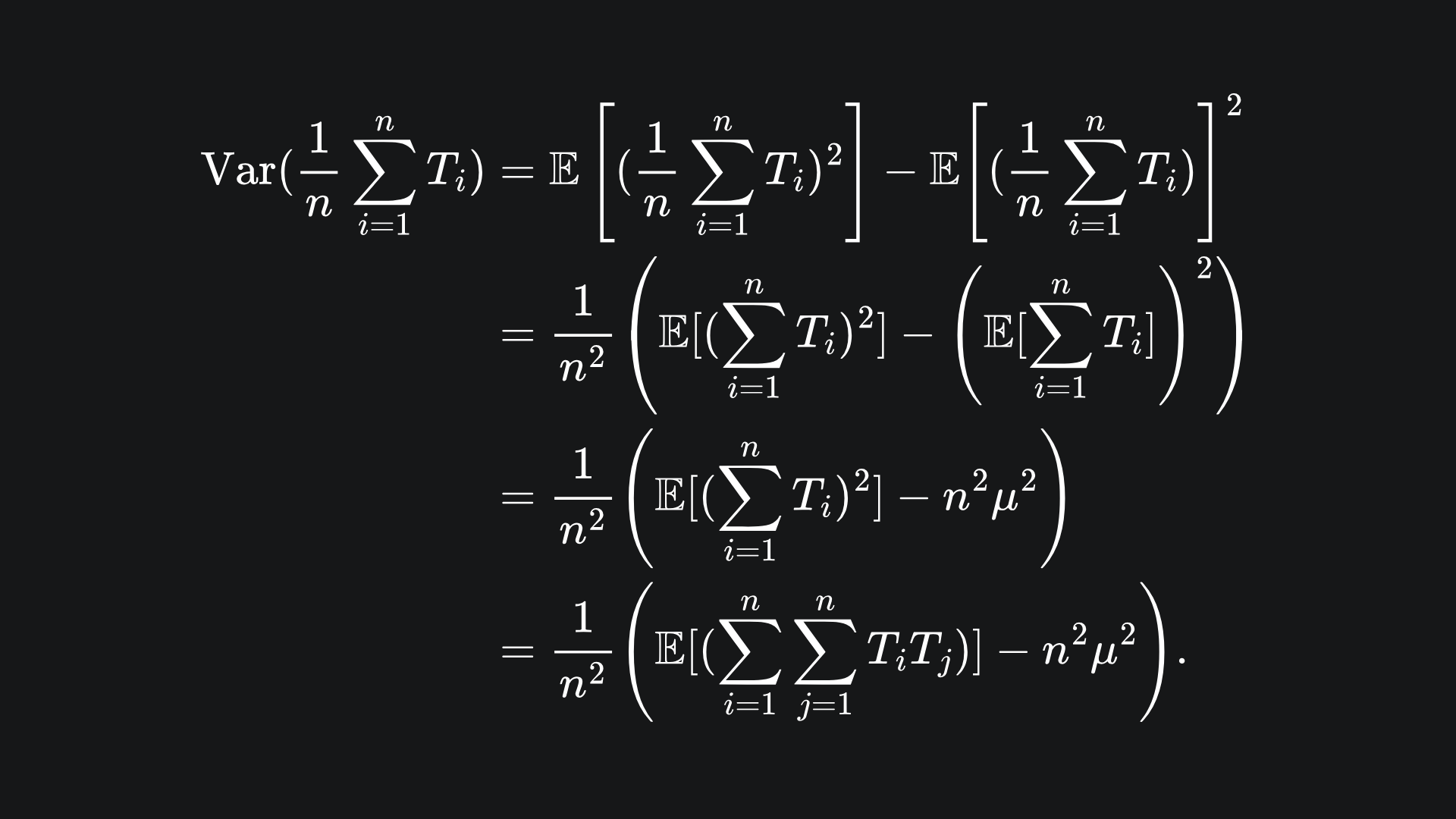
By the result (*) we have that
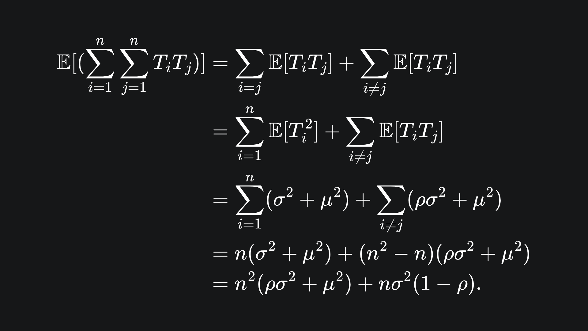
Substituting this into the variance formula gives us
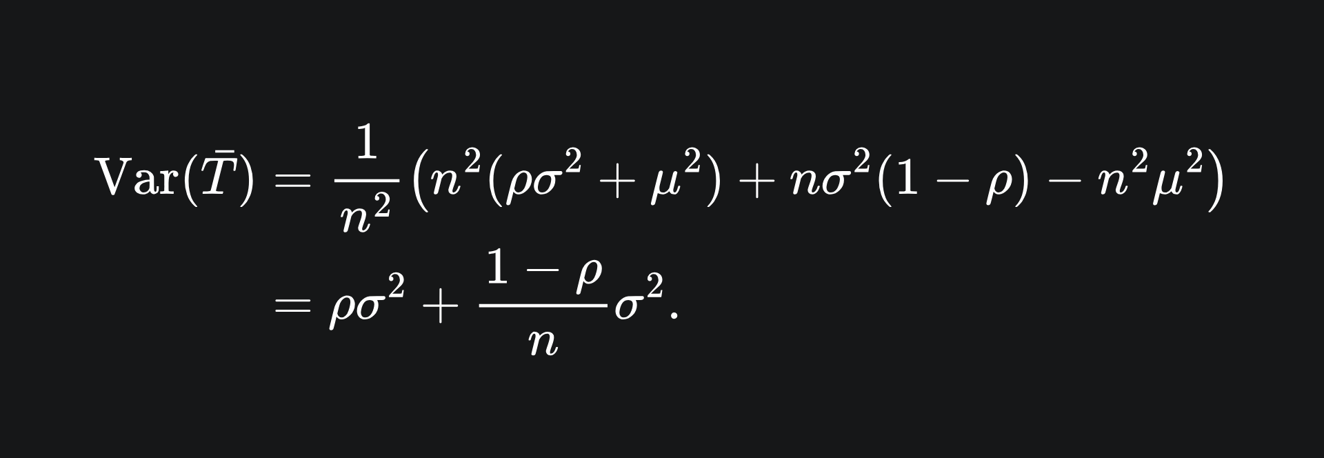
And that concludes the proof!
I realise that I haven’t actually defined what bias is in the context of ML. I’ll try and write about the bias-variance trade-off at some point in the future.