
The Upper Confidence Bound (UCB) algorithm for MAB problems
Explaining how the 'optimism under uncertainty' principle can be used to solve the MAB problem.

Hello fellow machine learners,
Last week, we continued our discussion of Multi Armed Bandits by breaking down the successive elimination algorithm and used Hoeffding’s inequality to construct confidence intervals for the rewards of each arm. Be sure to read that article before this one:
Today, we will be doing a deep dive into the Upper Confidence Bound algorithm for MAB.
Make sure you’re strapped in, because it’s time to unpack!
The UCB algorithm
We can break the algorithm down into two main steps:
💡 To begin, we play each arm once.
💡 The arm that we select in the next round of the game is the arm with the current largest upper confidence bound. The UCB of the arm i is defined as
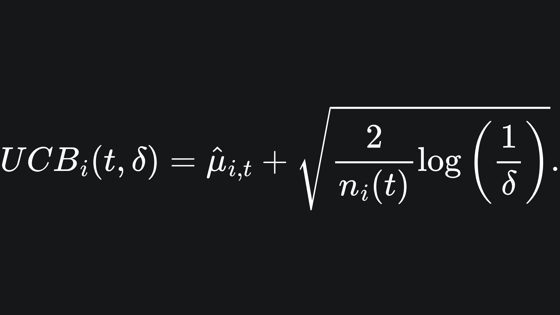
I think of this as the empirical mean reward with a ‘half interval’ of confidence added to it. This is similar to the confidence interval formulation we used last week.
Anyway, we can use the UCB values of round t to determine our arm choice in round t+1:
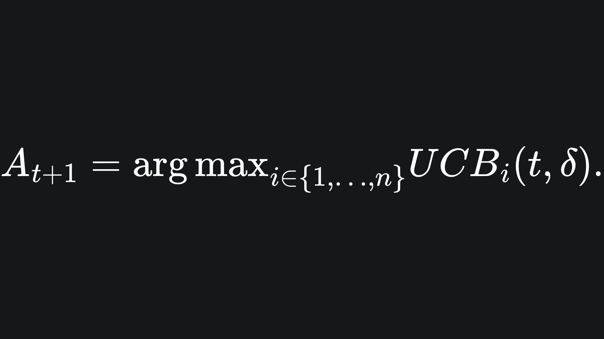
This is the formulation we use for the remaining rounds of the game.
Why the upper confidence bound?
This algorithm operates under the idea of ‘optmism under uncertainty’- we assume that the true mean reward of each arm is equal to the corresponding UCB value.
But this may sound somewhat counterintuitive, at least it did to me when I first learnt about this algorithm. After all, would we not want to make more conservative guesses about the true mean values, perhaps with the lower confidence bounds instead?
Well, a large value for UCBi(t, δ) will probably mean one (or perhaps both) of the following:
💭 The size of the half interval for arm i is large. This will happen if ni(t) is small, which is the case if arm i has not been explored much. In this case, it would be advantageous for us to play arm i more often, to help us become more confident about the true mean reward of arm i.
💭 Arm i yields a large empirical reward, i.e. μ̂i is large. In this case, we would want to play arm i more anyway in order to maximise our gains across the rounds.
Visualisation
Here is an example of the UCB algorithm in action (now with audio!):
We observe that, although the green arm is played often initially, the decrease in size of the corresponding half interval allows the purple arm’s UCB to come into play more in the later rounds. It just so happened that the green arm yielded unusually large rewards in this simulation, but the algorithm still managed to work things out with enough rounds. You can try the code out for yourself by changing the arm reward distributions, numpy random seed and more here.
Packing it all up
And that’s a wrap! The mathematics we built up in the previous two articles saved us a lot of heavy lifting this time round. Here is the usual roundup:
💡 The Upper Confidence Bound algorithm assumes that the true mean rewards are at the upper confidence bound of the empirical mean rewards.
💡 We operate under this ‘optimism under uncertainty’ principle, because a large UCB value means that we have either not played a particular arm much, or that it has a large empirical mean reward (or both!).
💡 Similar to the successive elimination algorithm, one can play around with the parameter δ to control the overall half interval sizes.
Training complete!
I hope you enjoyed reading as much as I enjoyed writing 😁
Do leave a comment if you’re unsure about anything, if you think I’ve made a mistake somewhere, or if you have a suggestion for what we should learn about next 😎
Until next Sunday,
Ameer
PS… like what you read? If so, feel free to subscribe so that you’re notified about future newsletter releases:
Sources
My GitHub repo where you can find the code for the entire newsletter series: https://github.com/AmeerAliSaleem/machine-learning-algorithms-unpacked
“Reinforcement learning: An Introduction”, by Richard S. Sutton and Andrew G. Barto: https://web.stanford.edu/class/psych209/Readings/SuttonBartoIPRLBook2ndEd.pdf (^ btw this is a GOATed resource for RL in general)
“Bandit Algorithms”, by Tor Lattimore and Csaba Szepesvari: https://www.cambridge.org/core/books/bandit-algorithms/8E39FD004E6CE036680F90DD0C6F09FC
Lecture notes on sub-Gaussian random variables: https://ocw.mit.edu/courses/18-s997-high-dimensional-statistics-spring-2015/a69e2f53bb2eeb9464520f3027fc61e6_MIT18_S997S15_Chapter1.pdf