
The Multivariate Gaussian distribution isn't as scary as you think
Explaining how the Multivariate Gaussian's parameters and probability density function are a natural extension of the one-dimensional normal distribution.
Hello fellow machine learners,
I’ll admit it: the Multivariate Normal distribution scared me when I first learnt about it during my undergraduate studies.
I had only just gotten used to the formula for the scalar normal distribution. Now all of a sudden, lecturers were throwing around vectors and matrices around like frisbees.
What is the Multivariate Normal distribution? What do its parameters mean? Why do we care about it?
We’ll answer the final question next week1, but for today, the goal is to justify why/how the MVN extends the scalar version in a very natural way.
(Even if I didn’t feel like that was the case at first myself 🤐)
You know the drill… let’s get to unpacking!
The normal distribution
The normal distribution is also known as the Gaussian distribution. This alternate name pays homage to Carl Friedrich Gauss, the man who came up with the distribution’s probability density function (pdf). You can read more about the distribution’s origins here. I’ll stick to saying ‘Gaussian’ for the most part, because it sounds cooler.
A random variable X is said to follow a Gaussian distribution of parameters (μ, σ2), written as X ~ N(μ, σ2) if its pdf is given by
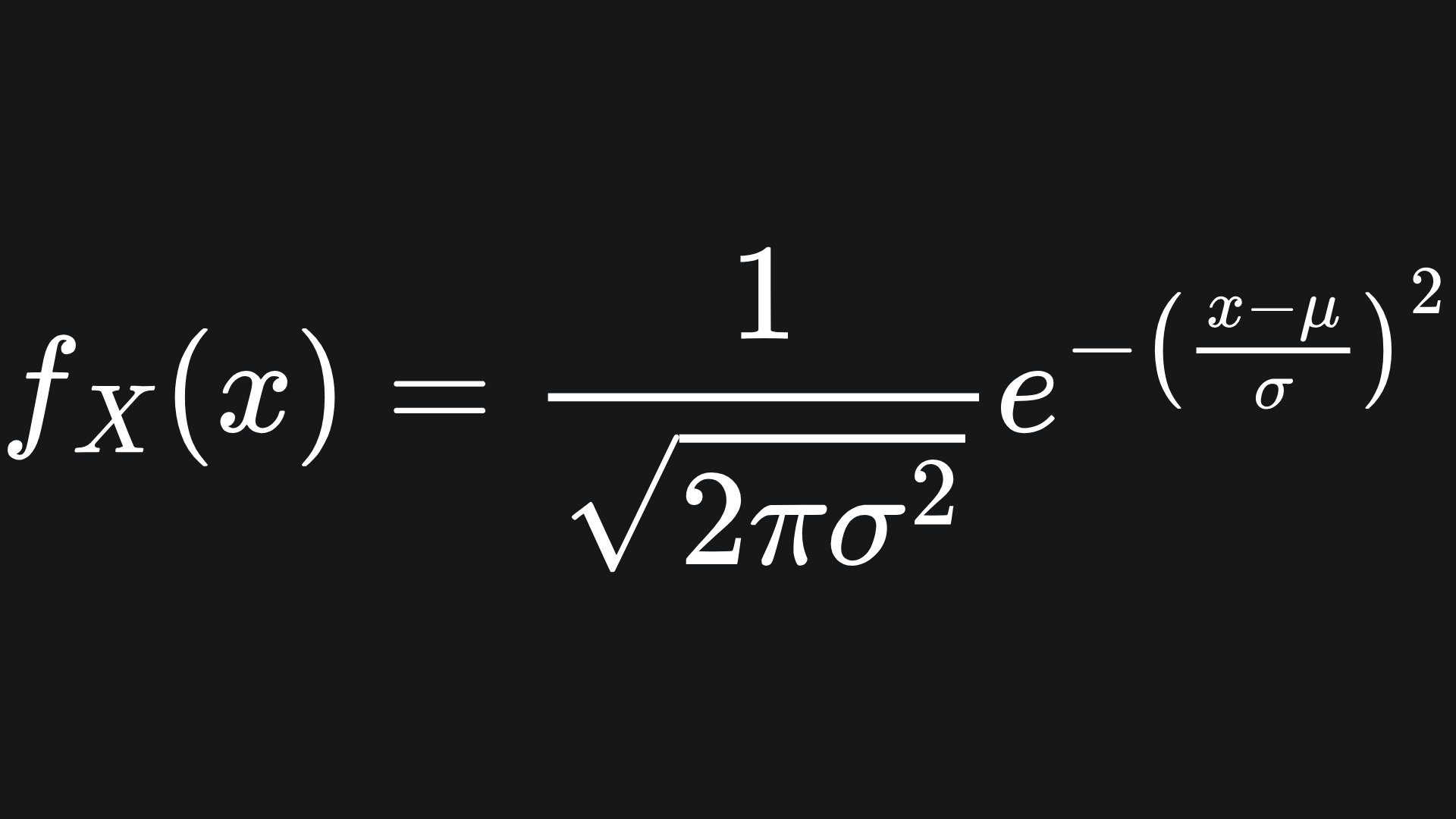
Statisticians love the Gaussian distribution for many reasons, which we could unpack in future articles2. For now though, just note that μ is the mean of the distribution and σ2 is its variance. One can think of σ2 as the spread of the distribution: the larger the value, the more spread out the values are.
The Multivariate Normal (MVN) distribution
A natural question for a mathematician like me is whether the the one-dimensional Gaussian distribution from the previous section can be extended to account for finitely many dimensions. This is where the Multivariate Gaussian comes in!
Rather than scalar mean and variance, the MVN is characterised by a mean vector μ and covariance matrix Σ. The mean vector is a natural extension of the scalar mean μ that we had before- the i-th entry of μ is simply the mean of the i-th data dimension.
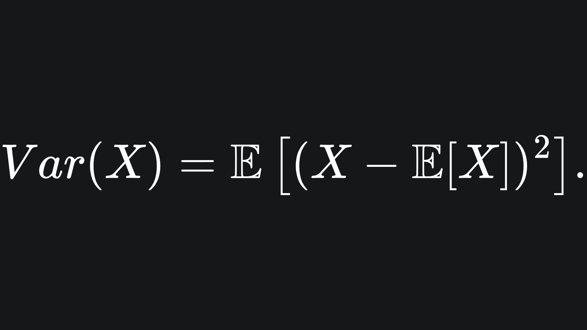
But where did the covariance matrix come from? It might not look like it, but in a similar way, the covariance matrix Σ is a natural extension of the scalar variance to n dimensions. Recall the statistical formula for variance, which takes one random variable as input and computes the ‘spread’ of its values from the mean:
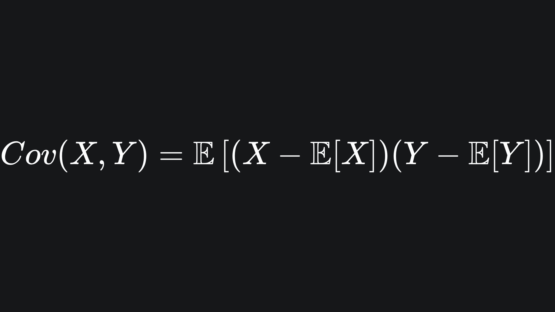
The covariance function takes a pair of random variables as input and measures the relationship between them. The formula is
Can you spot the connection? The variance of X is nothing more than the covariance between X and itself:
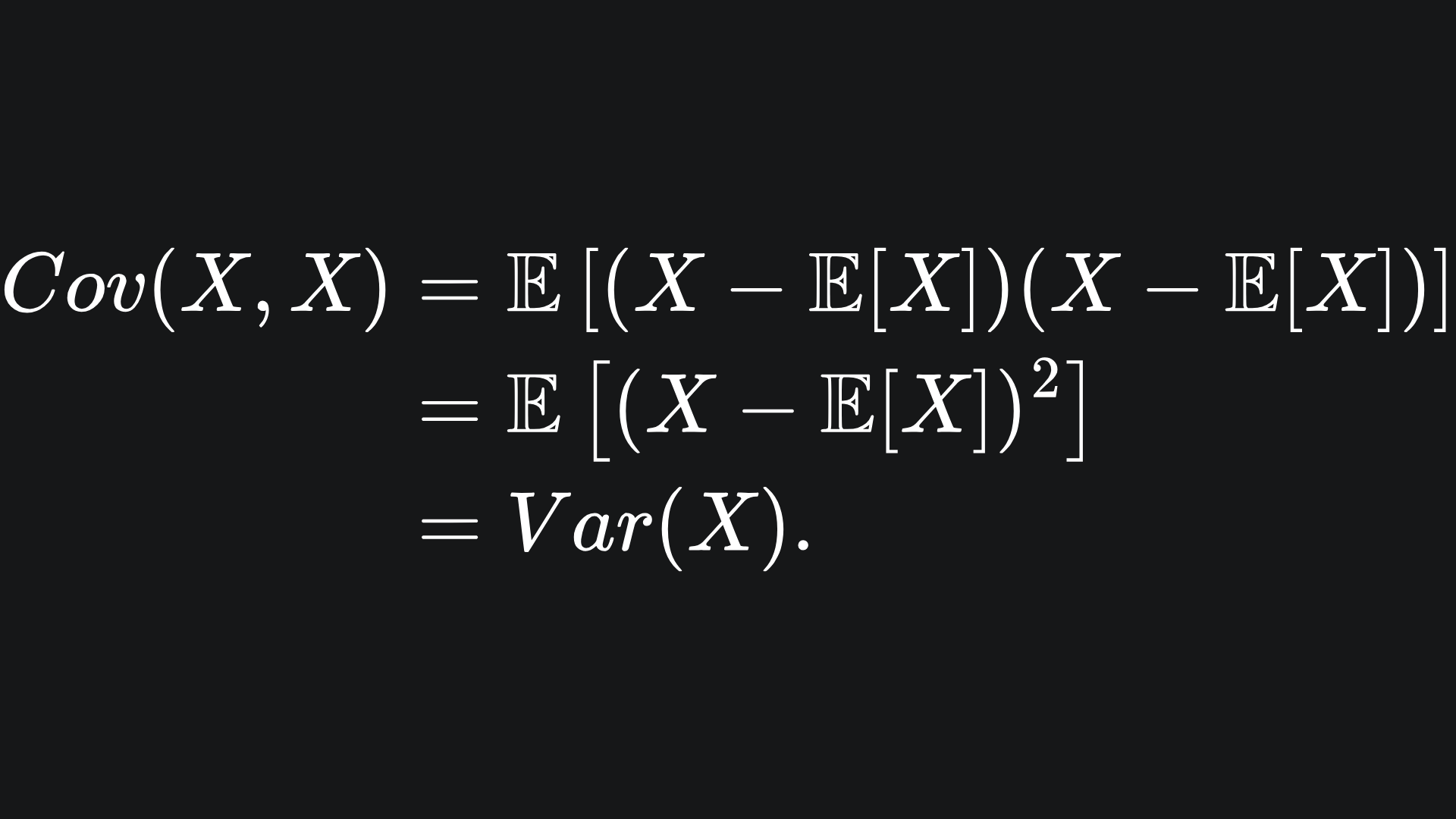
In the scalar Gaussian case, we are only working with one-dimensional data, and so the covariance formula collapses into variance by default.
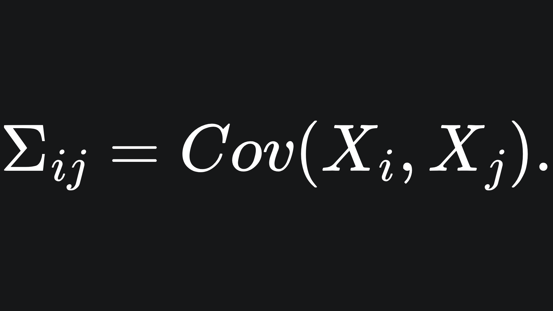
But for a random vector X=(X1, X2, … , Xn), we can measure the covariance between each pair of its elements. We can load these into a matrix, which is what the covariance matrix is: the (i,j)-th entry of the covariance matrix Σ is defined as
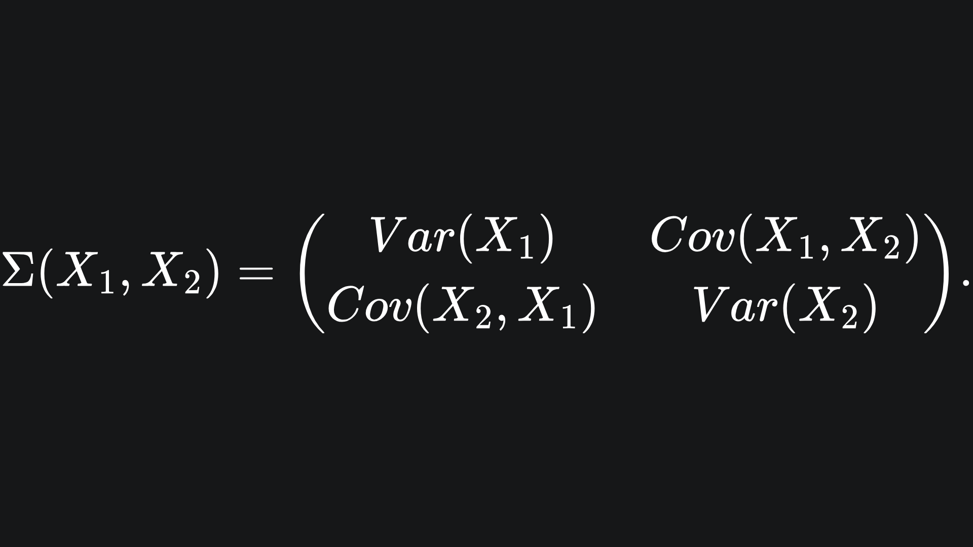
Note that the covariance function is symmetric, and so the covariance matrix is also symmetric. Moreover, the i-th diagonal is the variance of the i-th element of the random vector X. So in two dimensions for example, the covariance matrix for the random vector X=(X1, X2) will look like:
We say that the n-dimensional random variable X follows a Multivariate Gaussian distribution, i.e. that X ~ MVN(μ, Σ), if the pdf of X is given by
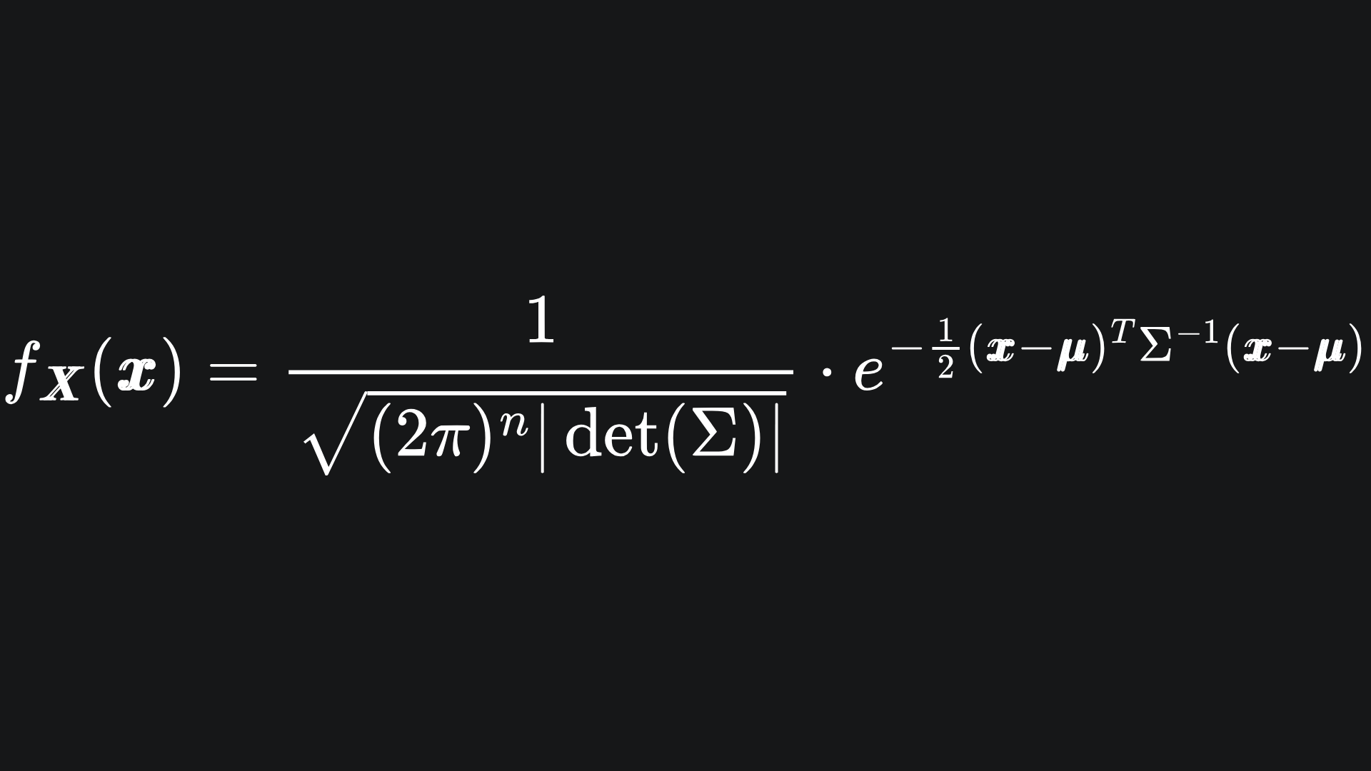
It might look like a car crash, but don’t panic! Just like any other pdf, it returns a scalar value. Let’s compare the univariate and multivariate formulas:
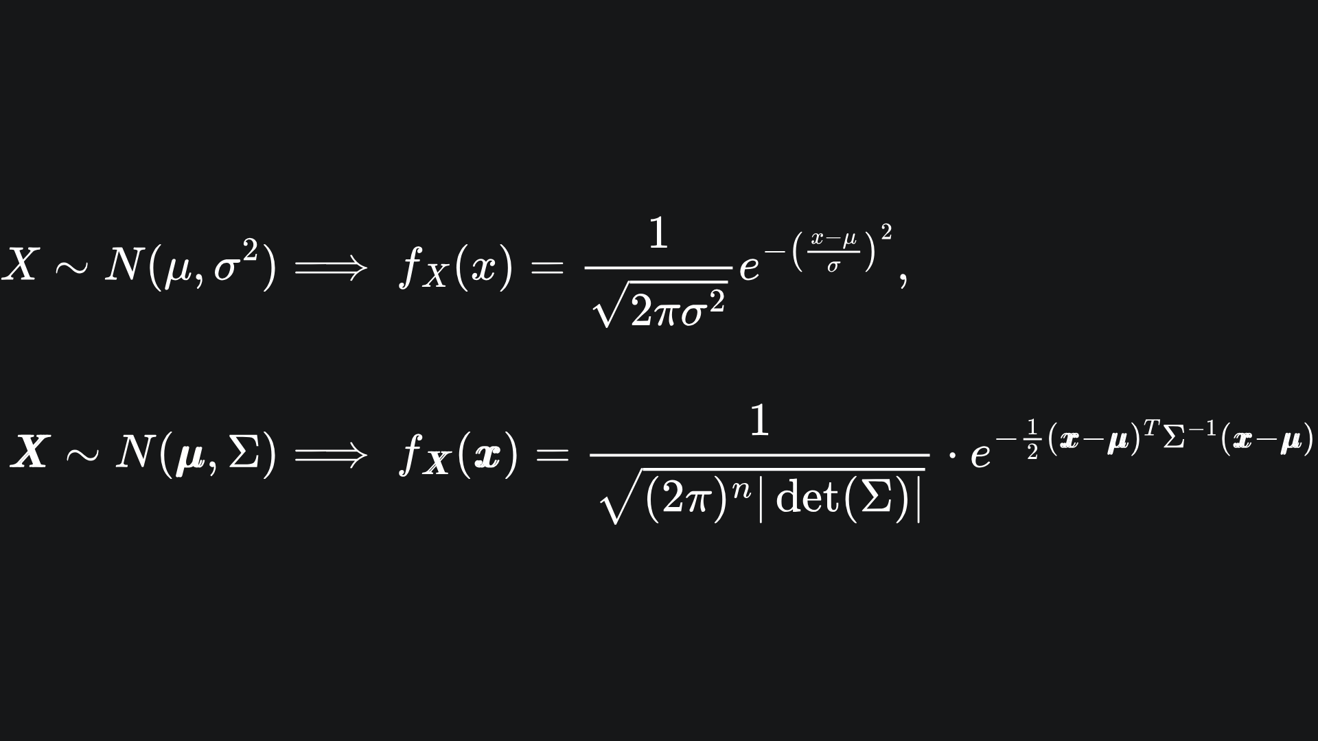
Well, there are certainly some similar flavours:
💡 The normalising constant in front follows a similar scaling that involves powers of 2π and the size of the (co-)variance.
💡 The 1d formula uses a power of two in the exponent, but in multiple dimensions this becomes the vector (X - μ) multiplied with its transpose. The product must begin with the transpose to ensure that we get a scalar value out at the end. But this essentially sums up the squares of the elements of the vector (X - μ). So indeed, a natural extension of the 1d case.
💡 The scalar 1/σ2 in the exponent becomes a matrix inverse for the multivariate pdf, namely Σ-1. The matrix inversion is the high-dimensional analogue of the division operation, similar to the vector-multipled-by-its-transpose concept in the previous point.
Visualisation
We will wrap up this discussion by showcasing the Multivariate Gaussian pdf for n=2 dimensions, which creates a surface in 3D:
We can see that changing the mean values acts to translate the Gaussian’s main bump, while modifications to the covariance matrix affect the shape of the bump. This aligns with the animation we had for the univariate distribution!
The GitHub repo here helped me put the code together for this week’s animation.
Packing it all up
Loads of theory in this week’s article, but its utility will be showcased in an ML algorithm we’ll discuss next time. Plus, good mathematical/statistical knowledge is an integral component of an ML practitioner’s toolkit. Here are the key insights from today:
🔑 The univariate Gaussian’s mean gives us some sense of translation, while its variance tells us about the spread of its values.
🔑 The Multivariate Gaussian aims to extend the the univariate distribution in the most natural way. Specifically, the mean parameter becomes a vector, while the variance decomposes into the pairwise covariances of the distribution’s elements, which are encoded in a (symmetric) matrix.
🔑 The probability density function for the Multivariate Gaussian looks pretty horrifying, but it is a natural extension of the pdf for the scalar distribution.
Training complete!
I hope you enjoyed reading as much as I enjoyed writing 😁
Do leave a comment if you’re unsure about anything, if you think I’ve made a mistake somewhere, or if you have a suggestion for what we should learn about next 😎
Until next Sunday,
Ameer
PS… like what you read? If so, feel free to subscribe so that you’re notified about future newsletter releases:
Sources
Manim code that helped me with the animation for the 2D Multivariate Normal pdf surface plot: https://github.com/t-ott/manim-normal-distributions/blob/master/bivariate.py
My own GitHub repo where you can find the code for the entire newsletter series: https://github.com/AmeerAliSaleem/machine-learning-algorithms-unpacked
A pleasant blog about origin of the Normal distribution: https://medium.com/@will.a.sundstrom/the-origins-of-the-normal-distribution-f64e1575de29
Online webpage about the covariance matrix: https://datascienceplus.com/understanding-the-covariance-matrix/
Since you bothered to pay attention to this footnote, I’ll just tell you- we’ll (hopefully) be discussing the Gaussian Mixture Model next week!
Let me know if this would be of interest!