Stochastic Gradient Descent vs Mini-batch descent for neural networks

Exploring how Stochastic Gradient Descent (SGD) and mini-batch gradient descent can help reduce the issues of good ol' standard gradient descent.

Hello fellow machine learners,

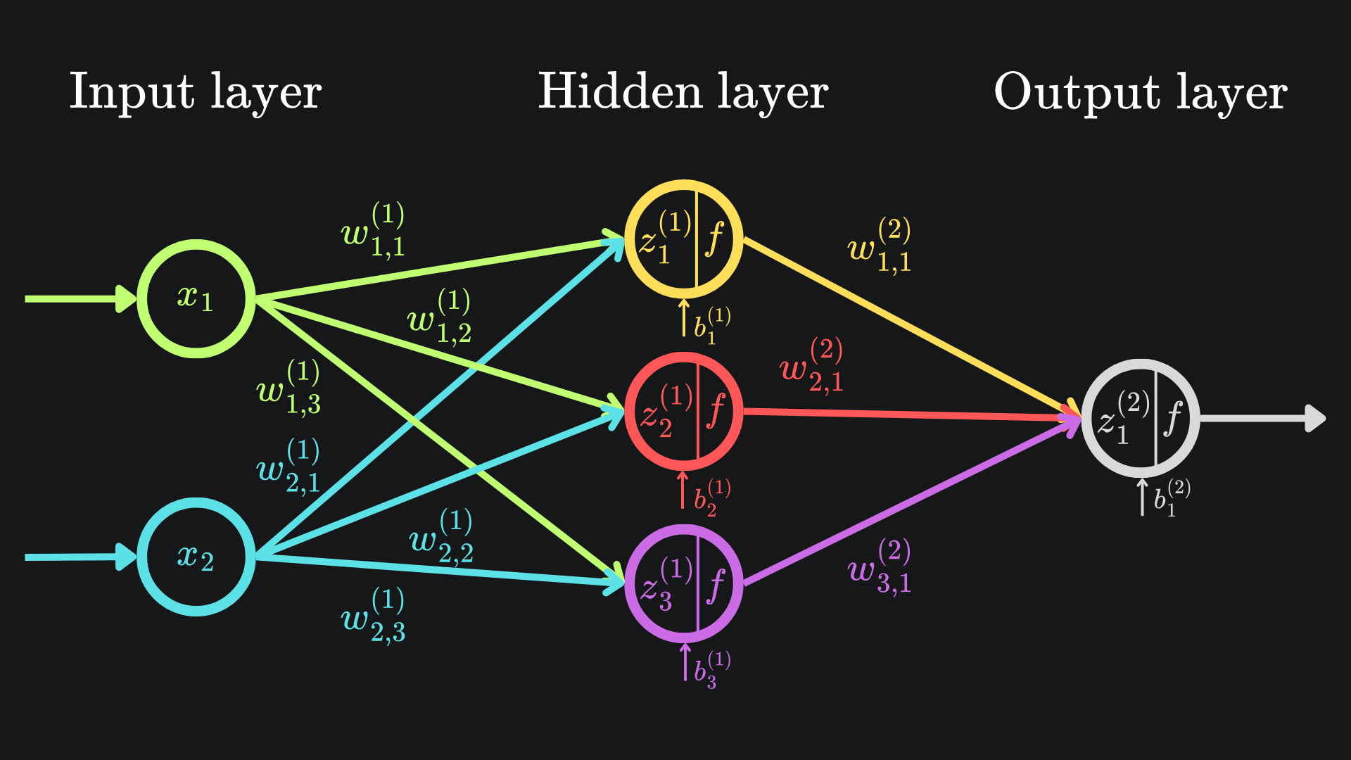
Last time, we explained how neural networks apply the backpropagation algorithm to learn. Crucially, we explored a pair of exemplar neural networks to show how the partial derivatives for later network parameters depend on the partial derivatives of earlier weights and biases.

That’s all well and good, but the sheer quantity of derivatives to keep track of became overwhelming very quickly. In particular, for our network of just six nodes, we ended up with 9 weights and 4 biases, with each of these 13 parameters having its own partial derivative expression. Here is what that network looked like:

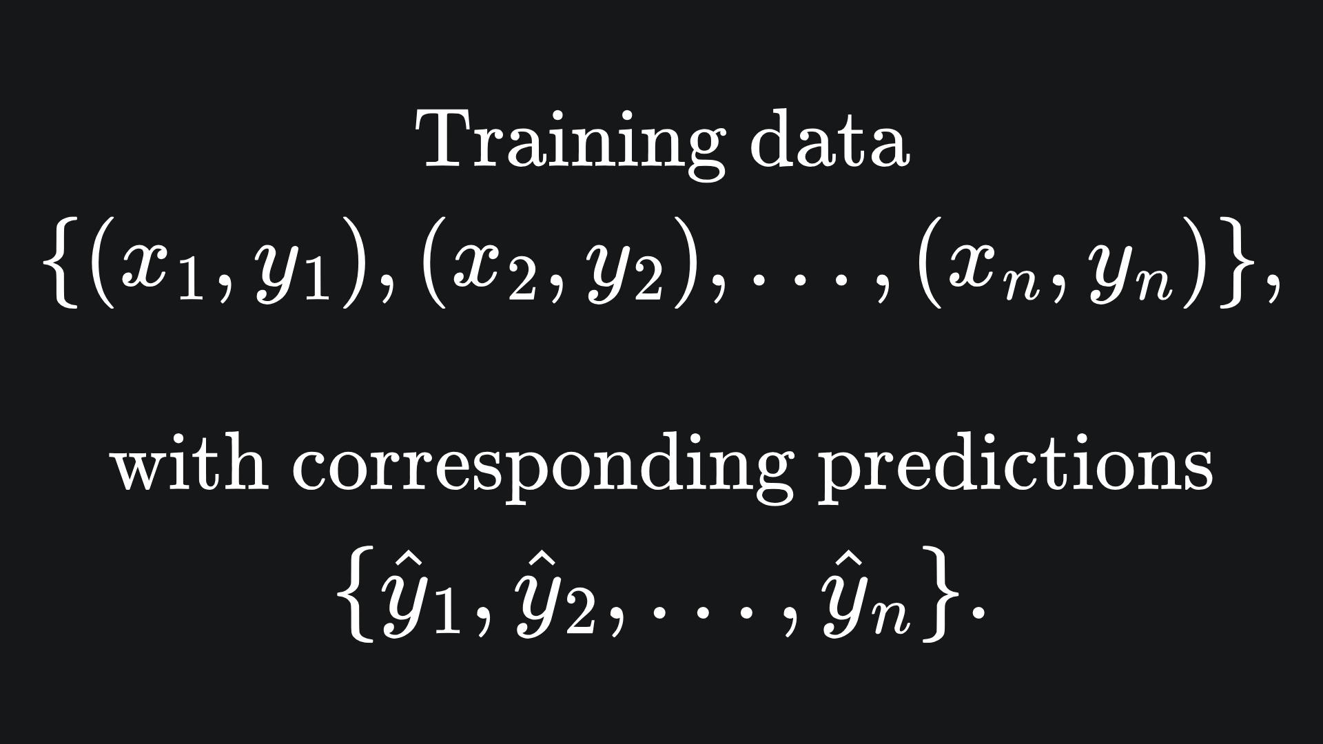
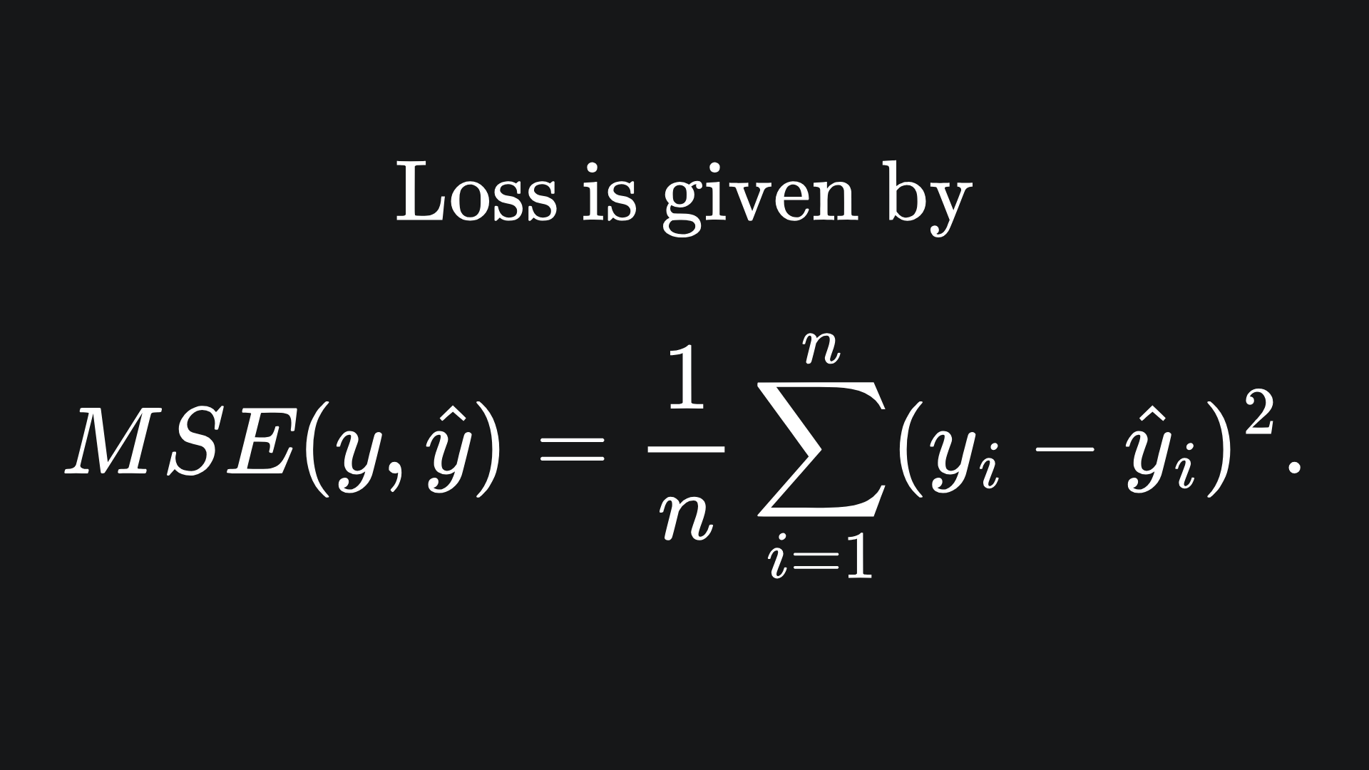
Moreover, the way I presented the backpropagation technique assumed the use of a single training datum. In particular, I used the Mean Squared Error (MSE) as the loss function of choice, but only plugged in one data point for its evaluation. In reality though, we needs lots of training data for the backpropagation technique to help a neural network to learn effectively. For example, instead of just taking the squared error between a single prediction and single label, we would have

And MSE would be applied to the set of predictions made on the training data, i.e.

These insights highlight two problems:

🤔 If our training set is very large, then we’ll need to use the network to make predictions for every data point and take the MSE of all these values. This means that the execution time of the forward pass scales up with the size of the training set.

🤔 The more network parameters we have, the more partial derivatives we’ll need to evaluate. Although some of them have similar expressions, the quantity and complexity of the partial derivatives can get out of hand very quickly.

Today, we’ll discuss a simple way of mitigating the former point, leaving the latter for another day.

Let’s get to unpacking!

Stochastic Gradient Descent (SGD)

A solution to running gradient descent on a large set of training data is to instead choose a single training point at random, generate the network’s prediction, and simply apply backpropagation on that. The nature of choosing an individual point from the training set is what makes this technique ‘stochastic’, hence the name of Stochastic Gradient Descent (SGD). Note that we choose a new data point at random for each step of the gradient descent.

So ironically, a solution to the problem is to just apply MSE, backpropagation, etc. to a single data point like we did in the last article!

Clearly, this reduces the runtime of the standard forward pass, because we’re now working with an individual input. However, there is one big issue with this approach: the gradient updates with SGD are more noisy in comparison to running the whole dataset through the algorithm. This is because it is not usually possible for one data point to represent the trends and patterns of the entire dataset, and so the updates to the network’s weights and biases won’t necessarily be to the benefit of general patterns. Such inaccuracies can affect model performance on unseen data points too. So while convergence can still happen with SGD, the value of the loss tends to fluctuate more erratically¹.

Another issue is with that of the learning rate. All gradient descent algorithms require a well-tuned learning rate, but the noisy updates of SGD only add to this sensitivity.²

Mini-batch Gradient Descent

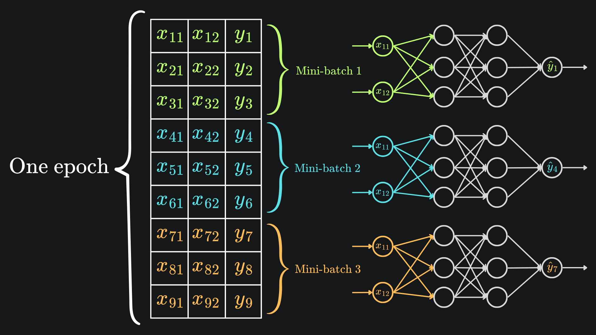
A more optimal technique lies in striking a balance between the two methods discussed thus far. Namely, we can split the data into ‘mini-batches’, by partitioning the training data into disjoint chunks. We can shuffle all the rows before partitioning the data to ensure that stochasticity remains present in the resultant mini-batches, and techniques like stratified sampling can help retain the global data trends within each mini-batch. Then, for each step of gradient descent, we can take a separate mini-batch at random and apply gradient descent to that. The following diagram highlights this in the simple case of 9 training data points, with a mini-batch size of 3:

A simple example of mini-batches of size 3 for training data with 9 data points.

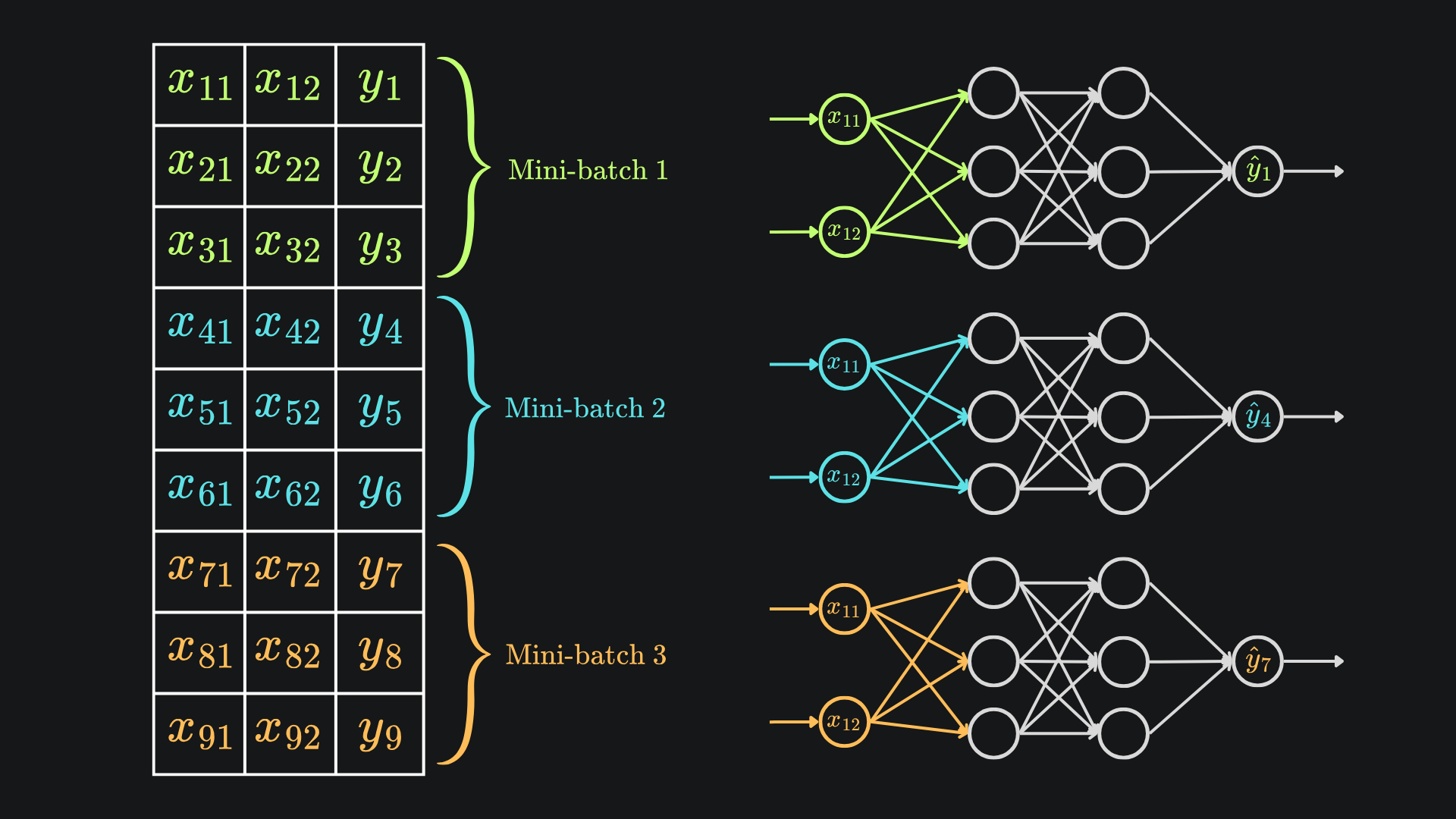
This once again reduces the complexity and runtime of an individual forward pass, but will help produce less noisy gradient updates when compared to standard SGD.

Epochs

In the context of our neural nets, an epoch is a complete pass of the entire training set through the gradient descent procedure. In order to train the network properly, we’ll need to leverage multiple epochs.

One step of standard gradient descent trains the model on one epoch by defintion. Conversely, for a training data of n points, you’d need to apply SGD n times to get through one epoch. Finally, for mini-batch gradient descent with a batch size of m, you would need at least n // m gradient steps to get through one epoch.

And here is an updated version of the previous diagram to put this into perspective:

Packing it all up

There is plenty more to be discussed about the different methods of gradient descent, but I hope that this article provides a good starting point. Here’s a roundup of the main points:

📦 The standard gradient descent algorithm uses the entire set of training data for each step, equivalent to one full epoch per gradient step. This allows for more stable convergence to the network’s minimum loss value. However, it is not efficient in terms of computer memory or computational resources: in terms of the former, the whole training dataset will most likely need to be stored in memory; and as for the latter, the forward pass computations inflate in line with the size of the training data.

📦 Stochastic Gradient Descent (SGD) sacrifices optimal gradient steps for the sake of efficiency, by using only one randomly selected data point for each gradient step. As such, this makes each descent step noisier, and so the choice of learning rate becomes all the more important.

📦 Mini-batch gradient descent divides the training data into random subsets called ‘mini-batches’. From then on, each gradient step uses one randomly selected mini-batch. This technique helps strike a balance the two previous methods, and the choice of mini-batch size can help skew this method to either performance or efficiency.

Training complete!

I hope you enjoyed reading as much as I enjoyed writing 😁

Do leave a comment if you’re unsure about anything, if you think I’ve made a mistake somewhere, or if you have a suggestion for what we should learn about next 😎

Until next Sunday,

Ameer

PS… like what you read? If so, feel free to subscribe so that you’re notified about future newsletter releases:

Sources

• My GitHub repo where you can find the code for the entire newsletter series: https://github.com/AmeerAliSaleem/machine-learning-algorithms-unpacked

1. More noise isn’t always a bad thing though, because it can help us escape local minima that standard GD may be more susceptible to.

2. The learning rate can be dynamically update to combat this, but more on that another day.