Optimising the Support Vector Machine using Lagrange multipliers (step-by-step breakdown)

Defining "constrained optimisation", how to solve such problems, and how this idea can be applied to the SVM.

Hello fellow machine learners,

Last week, we explored the vector tools needed to prove the formula for the margin of the Support Vector Machine.

This week, we’ll be, er, still talking about the SVM.

(Hope you’re not getting bored 👉🏼👈🏼)

Namely, we will talk about how to actually solve the constrained optimisation problem we set up in our first SVM article for the optimal separating hyperplane for our data, using some surprisingly powerful calculus techniques.

This article will be quite maths-heavy. Definitely make sure you’ve read the previous two SVM articles (first and second). It may also help to take a look at my articles on linear regression (here and here) to get a feel for how I set up ML problems mathematically.

Quadratic optimisation problem

We’re starting this article off with a deep dive into optimisation theory.

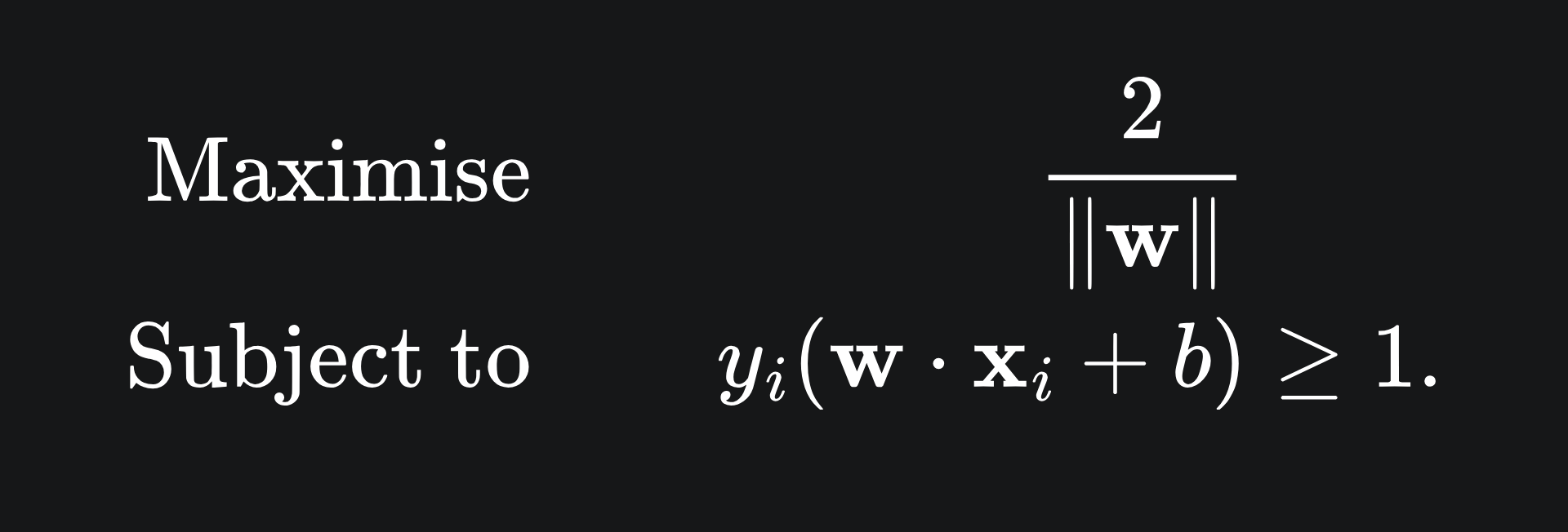
We have already covered the constrained optimisation problem whose solution will give us the optimal SVM hyperplane. Here’s a quick reminder:

\(\begin{align} \text{Maximise} & & \frac{2}{\|\textbf w\|} \\ \text{Subject to} & & y_i(\textbf w \cdot \textbf x_i + b) & \geq 1. \end{align}\)

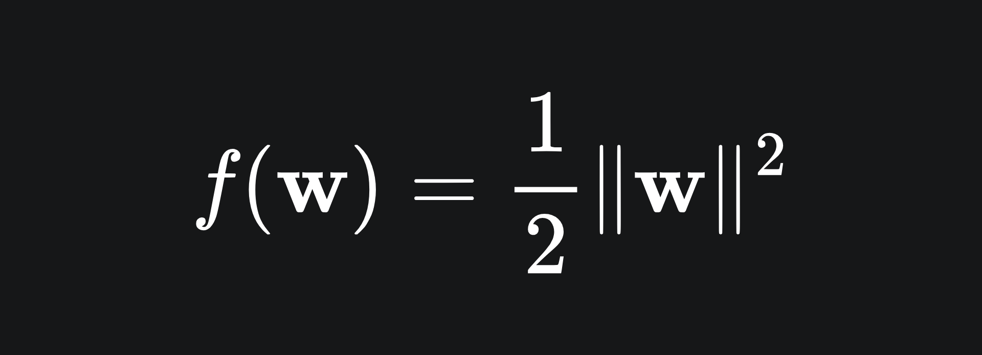
We will perturb the problem to make it a quadratic minimisation problem, for reasons that’ll become clear later on. Namely:

\(\text{Maximise } \frac{1}{\| \textbf w \|} \iff \text{Minimise } \| \textbf w \|^2.\)

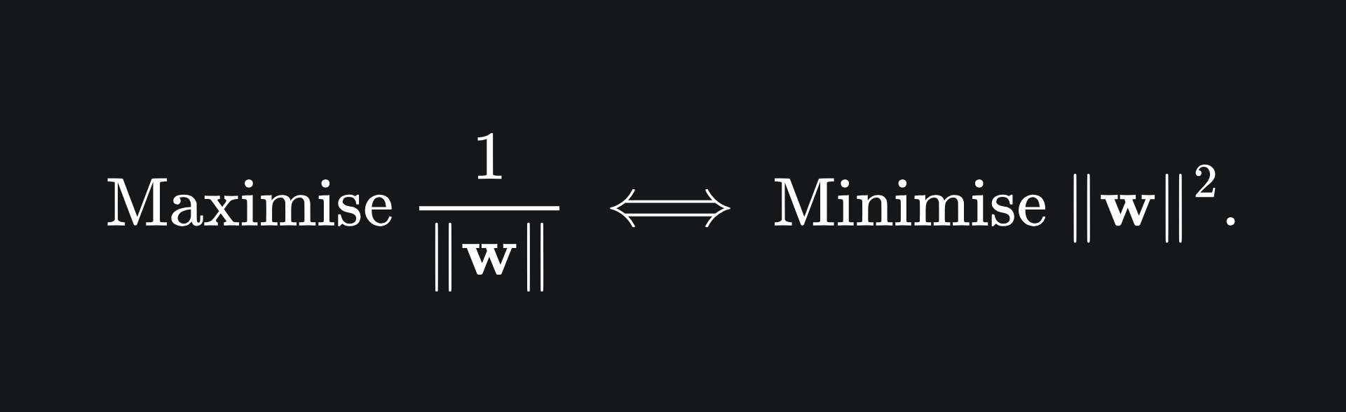
That is to say, rather than maximising the reciprocal of |w|, we instead aim to minimise the square of |w|.

This slight change to our objective is useful, because the square function is smooth, meaning we can differentiate it with ease. This leaves us with the quadratic optimisation problem, which we will refer to now as (M):

\(\begin{align} \text{Minimise } & & \frac{1}{2}\| \textbf w \|^2 & & \text{(M)} \\ \text{Subject to } & & y_i \cdot (\textbf w \cdot \textbf x_i + b) & \geq 1. \end{align}\)

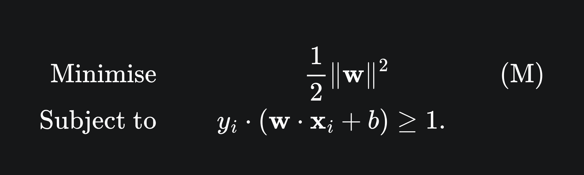
Notice that we have divided the objective by 2. This simply helps make the differentiation a tad simpler and does not really affect our goal.

So in order to find the optimal SVM, we need to find values (w*, b*) such that the objective function in (M) is minimised, yet the inequality in (M) is still satisfied by (w*, b*).

What does ‘constrained optimisation’ even mean?

Let’s try and understand this with an example of minimising a function subject to an equality constraint:

\(\begin{align} \text{Minimise} & & f(x,y) & =x^2+y^2 \\ \text{Subject to} & & g(x,y,z) & =x-z+1=0. \end{align}\)

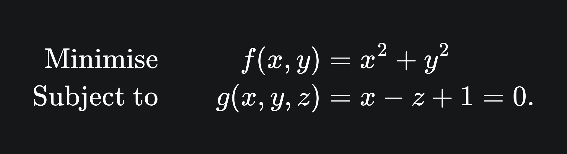
In words, this means that we want to find the values (x*, y*) that minimise the value of f, while ensuring that g(x*, y*) = 0. The function f gives us a paraboloid (blue) and the function g gives yields a plane (green):

To find (x*, y*), we will look at the contours of the function f. Just like a geographical map, the contours of a function are the sets of points at which f has the same height. These are also known as the level sets of f. A few level sets are shown as the yellow rings on the function f.

To minimise f subject to the constraint g, we look for the lowest point on f that intersects the plane g. This happens precisely at the level set that g is tangent to. This is depicted as the red level set below, and the optimal point in question is the orange dot:

The gradient of a function at a point is always perpendicular to the level set that the point lies on. This means that g is tangent to a level set when the gradient of g is parallel to the gradient of the paraboloid f. The blue arrow is the gradient of f at the point, and the green arrow is the gradient of the plane g:

Although the two arrows are pointing in opposite directions, they are still parallel.

This means that we can find the solution to the constrained optimisation problem if we find the point at which the gradients of the objective and constraint are parallel.

Here is the full-length animation in case you want to see all the steps in one:

Lagrange multipliers

Now that we have the visual intuition, let’s formulate this mathematically. We are looking for the point where the gradients of f and g are parallel. So we are looking for the point which satisfies

\(\begin{align} & \nabla f(x,y) = \lambda \nabla g(x,y) \\ \implies & \nabla f(x,y)-\lambda\nabla g(x,y)=0 \\ \implies & \nabla (f(x,y)-\lambda g(x,y)) = 0. \end{align}\)

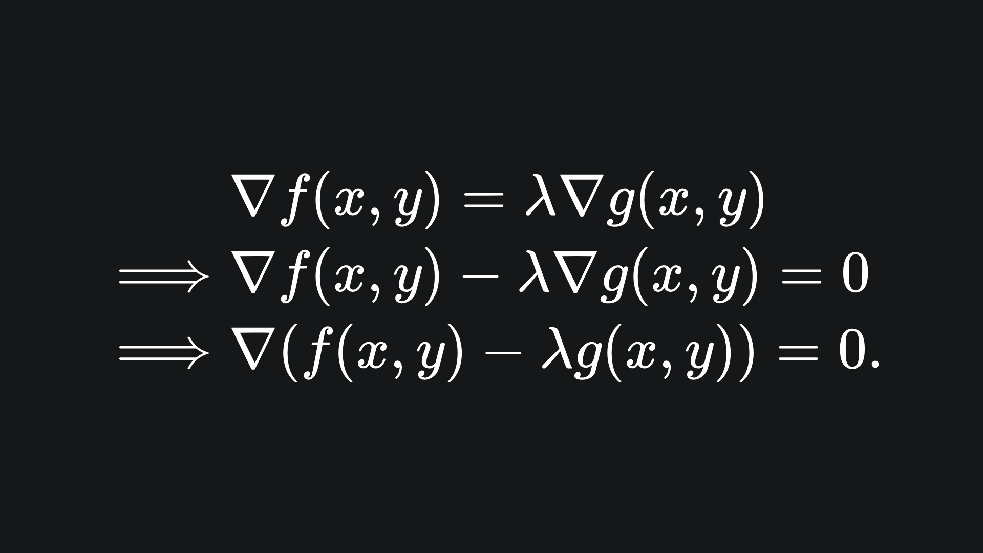
In the above, λ is called the Lagrange multiplier of the problem. The idea is to write out λ is terms of (x,y) and then solve for the optimal (x*, y*). The number of Lagrange multipliers will be equal to the number of constraints.

Optimisation with inequality constraints

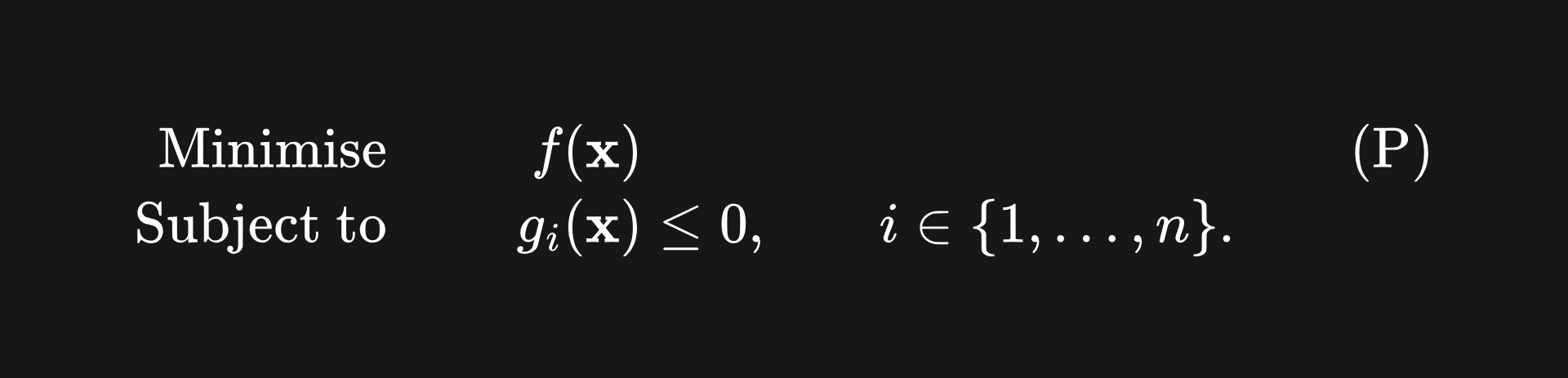
The good news is that we can apply the Langrange method to find an explicit solution for problems of the form (P) given below, where we have inequality constraints rather than just equality. The bad news is that I cannot explain it all in one article, so this next section is going to feel a lot like “oh just follow this recipe and ta-da!”. But bear with me all the same. We begin with the Lagrange primal problem

\(\begin{align} \text{Minimise } & & f(\textbf x) & & & & \text{(P)} \\ \text{Subject to } & & g_i(\textbf x) & \leq 0, & i \in \{1,\dotsc, n\}. \end{align}\)

To solve this kind of problem, we define the Lagrangian (L) to be

\(\begin{align} \mathcal{L} (\textbf{x}, \pmb{\alpha}) = f(\textbf x) + \sum_{i=1}^n \alpha_i g_i(\textbf x). & & \text{ (L)} \end{align}\)

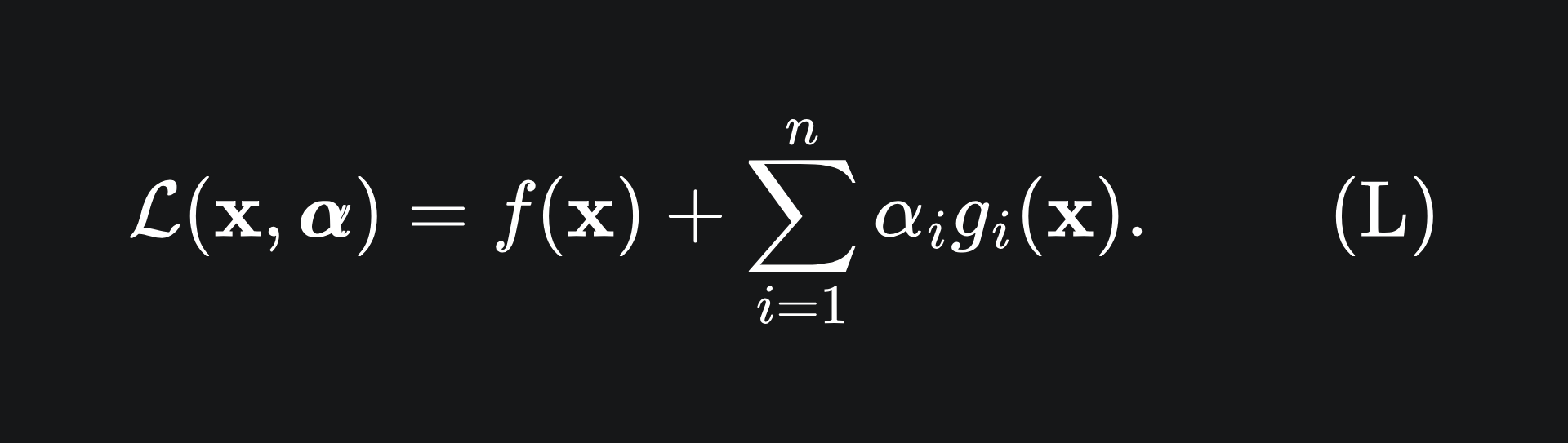
The vector α = (α_1,…,α_n) consists of the so-called Lagrange multipliers for the problem.

Thus far, this is pretty much the same as the example we provided in the previous section. But here is where we follow the recipe and I ask that you trust me.¹

Our goal is to maximise the value of the Lagrangian with respect to the Lagrange multipliers α. This gives rise to the Lagrange primal, which we can write as

\(L_p(\textbf x) = \sup_{\pmb{\alpha} \geq \textbf 0} \{ \mathcal{L}(\textbf x, \pmb{\alpha}) \}.\)

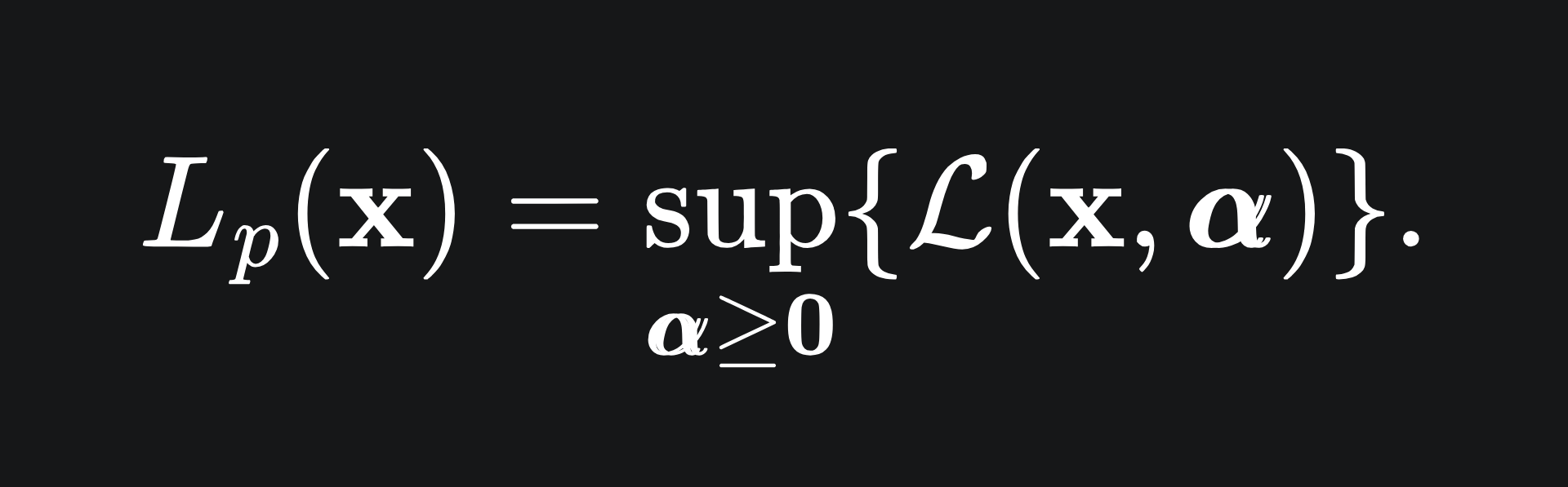
We are taking the supremum over non-negative α, because g_i(x) <= 0 for each i as part of our constraints. If any of the constraints are violated, e.g. g_i(x) > 0 for some i, then (L) shoots off to infinity; we could just take α_i to be as large as we like for that specific value i.

However, when the constraints are satisfied, the Lagrange primal becomes

\(\begin{align} L_p(\textbf x) & = \sup_{\pmb{\alpha} \geq \textbf 0} \left\{ f(\textbf x) + \sum_{i=1}^n \alpha_i g_i(\textbf x) \right\} \\ & = f(\textbf x) + \sup_{\alpha_1,\dotsc,\alpha_n \geq 0} \left\{ \sum_{i=1}^n \alpha_i g_i(\textbf x) \right\}. \end{align}\)

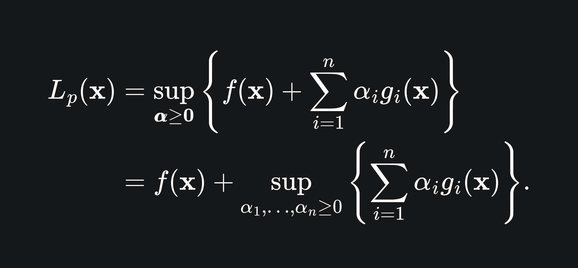
Since we have stipulated that α >= 0, with constraints g_i <= 0, the second term can be at most 0, and so the value of the Lagrange primal coincides precisely with the value of f(x) in this case. Therefore, minimising this quantity over all x will give us the solution we want! We define this to be the optimal value for the primal problem:

\(p^* = \inf_{\textbf x} \{ L_p(\textbf x) \}.\)

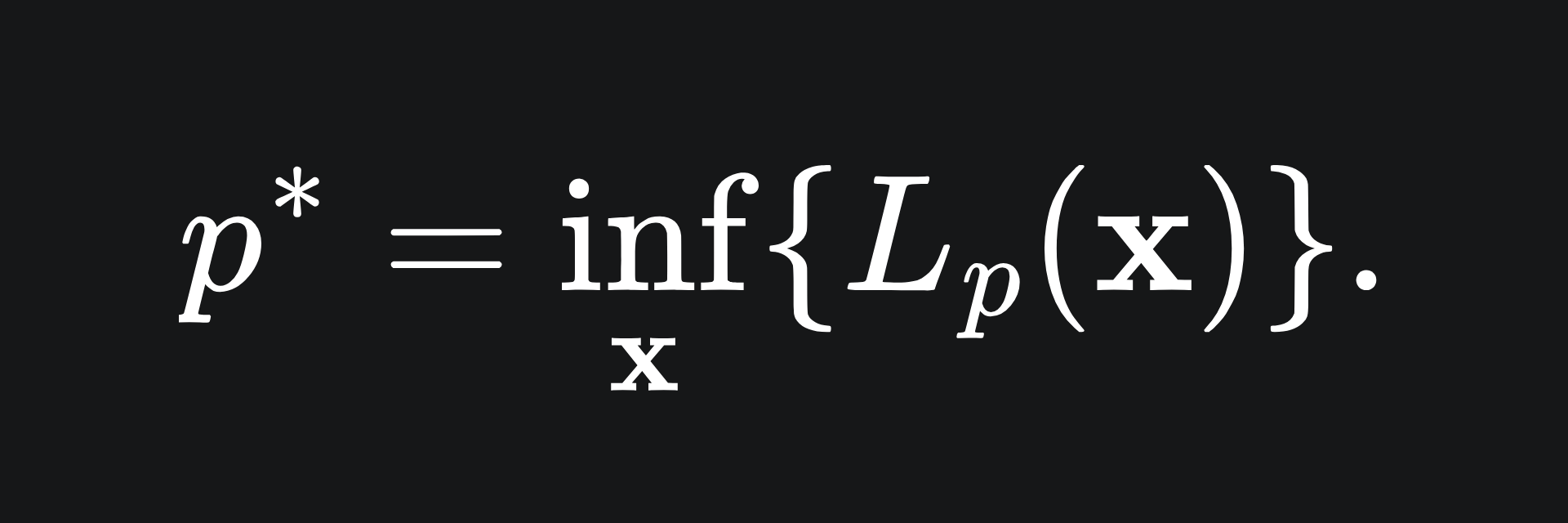
That is to say, the value p* is the solution to the original problem (P).

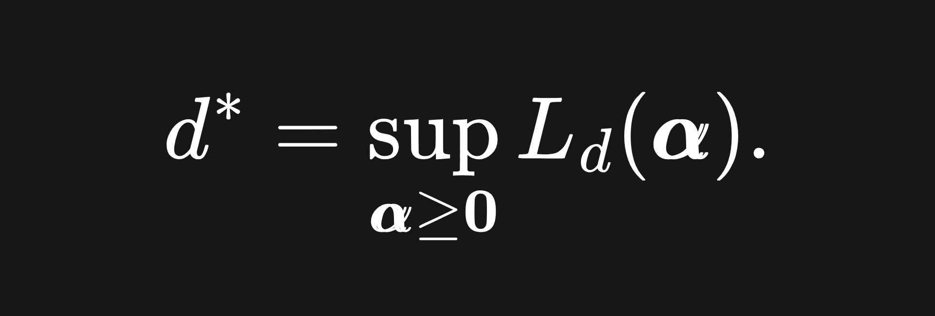
Now to twist this around: what happens if we minimise over x first and then then maximise over our Lagrange multipliers α after? Written explicitly, we define the Lagrange dual to be

\(L_d(\pmb \alpha) = \inf_{\textbf x} \mathcal L(\textbf x, \pmb \alpha),\)

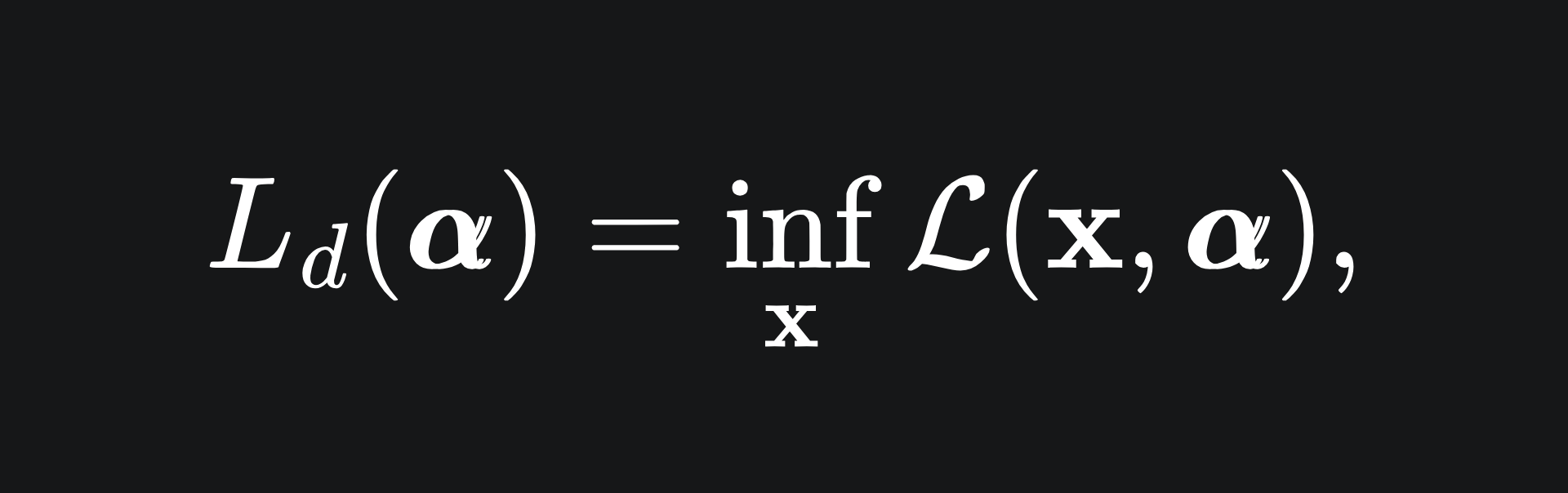
the dual problem as

\(\begin{align} \text{Maximise } & & L_d(\pmb \alpha) \\ \text{Subject to } & & \alpha_i \geq 0, & & i\in\{1,\dotsc,n\}. \end{align}\)

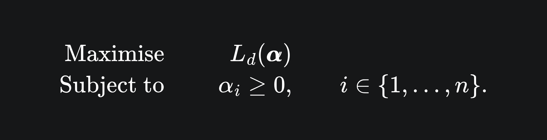
and the optimal value for the dual problem:

\(d^* = \sup_{\pmb \alpha \geq \textbf 0} L_d(\pmb \alpha).\)

Under certain conditions (i.e. not always²), we have that p*=d*. We shall use the dual problem instead of the primal problem to acquire the optimal (w*, b*) for our SVM, for reasons that will become clear later/next week.

Here is how we’ll use the above for the SVM problem:

1. Set up the Lagrangian for the SVM constrained optimisation problem.

2. Minimise the Lagrangian with respect to the hyperplane’s parameters (w, b), which will be expressed in terms of α.

3. Substitute these back into the Lagrangian and maximise with respect to α to obtain the optimal α value.

4. Use the value of α* to recover our desired (w*, b*).

Applying the Lagrange method to the SVM

We shall now attempt the put the SVM problem into the form (P). We are trying to find the optimal hyperplane to separate our data, so x is essentially (w, b). With this in mind, the function f from the previous section is simply

\(f(\textbf w) = \frac{1}{2}\| \textbf w \|^2\)

and each function g_i is given by

\(\begin{align} g_1(\textbf w, b) = 1-y_1(\textbf w \cdot \textbf x_1 + b), \\ g_2(\textbf w, b) = 1-y_2(\textbf w \cdot \textbf x_2 + b), \\ \dotsc \\ g_n(\textbf w, b) = 1-y_n(\textbf w \cdot \textbf x_n + b). \end{align}\)

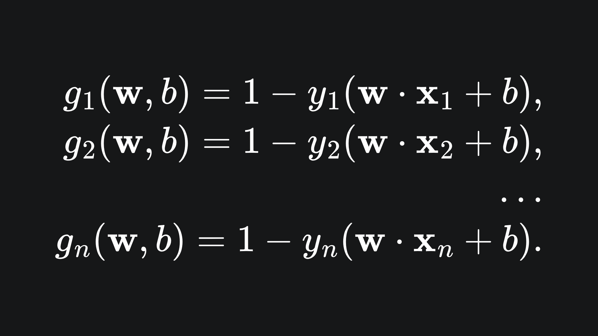
The reason we have written the constraints like this is so that

\(\begin{align} g_i(\textbf w, b) & \leq 0, & \forall i\in\{1,\dotsc,n\} \end{align}\)

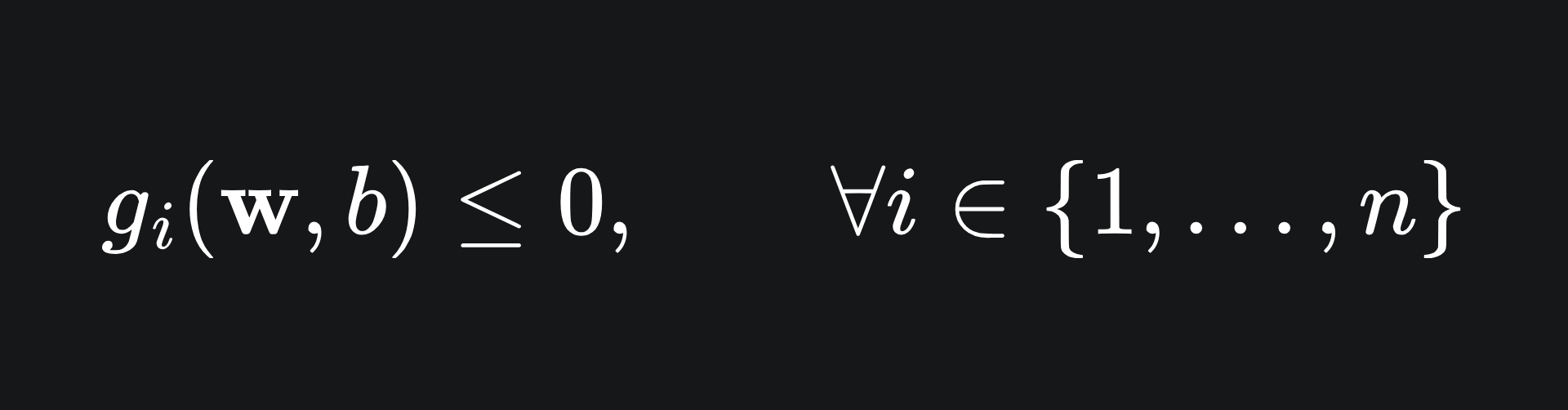
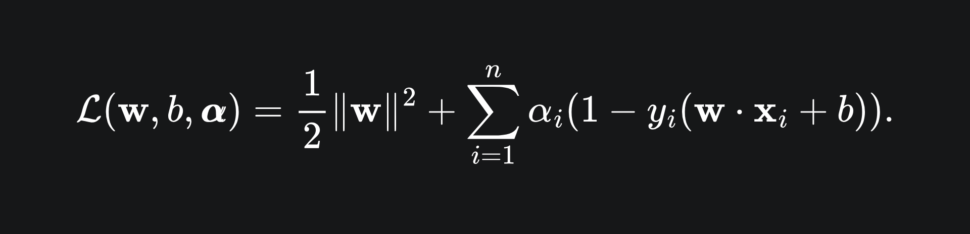
as specified in the problem setup (P). Consequently, the Lagrangian for the problem is given by

\(\mathcal{L} (\textbf w, b, \pmb{\alpha}) = \frac{1}{2}\| \textbf w \|^2 + \sum_{i=1}^n \alpha_i (1-y_i(\textbf w \cdot \textbf x_i + b)).\)

Nice! Following the dual problem formulation, we next need to differentiate the Lagrangian with respect to the SVM’s parameters. I’ll leave you to write out the details, so verify for yourself that

\(\begin{align} \frac{\partial \mathcal L}{\partial \textbf w} & = \textbf w - \sum_{i=1}^n \alpha_i y_i \textbf x_i \\ \frac{\partial \mathcal L}{\partial b} & = -\sum_{i=1}^n \alpha_i y_i \end{align}\)

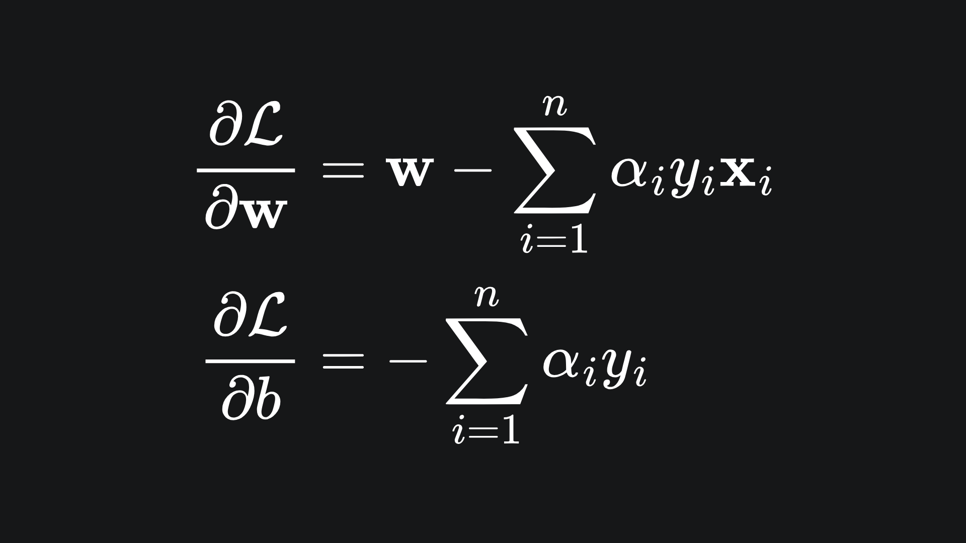
and that setting both of these to 0 leaves us with

\(\begin{align} \textbf w & = \sum_{i=1}^n \alpha_i y_i \textbf x_i, \\ 0 & = \sum_{i=1}^n\alpha_i y_i. \end{align}\)

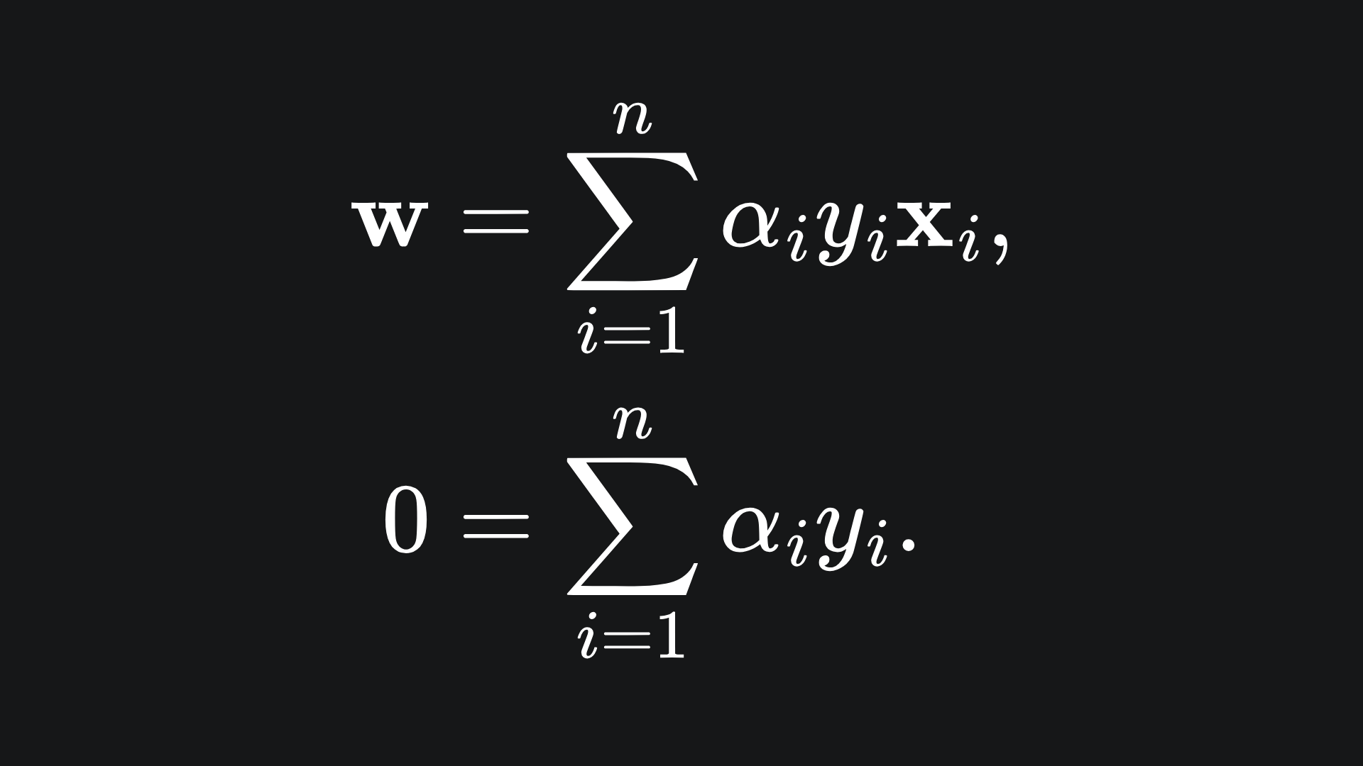
If you substitute these back into the Lagrangian, you should be left with

\(\mathcal L (\textbf w, b, \pmb \alpha) = \mathcal L (\pmb \alpha) = \sum_{i=1}^n \alpha_i - \frac{1}{2}\sum_{i=1}^n\sum_{j=1}^n\alpha_i\alpha_j y_i y_j(\textbf x_i \cdot \textbf x_j).\)

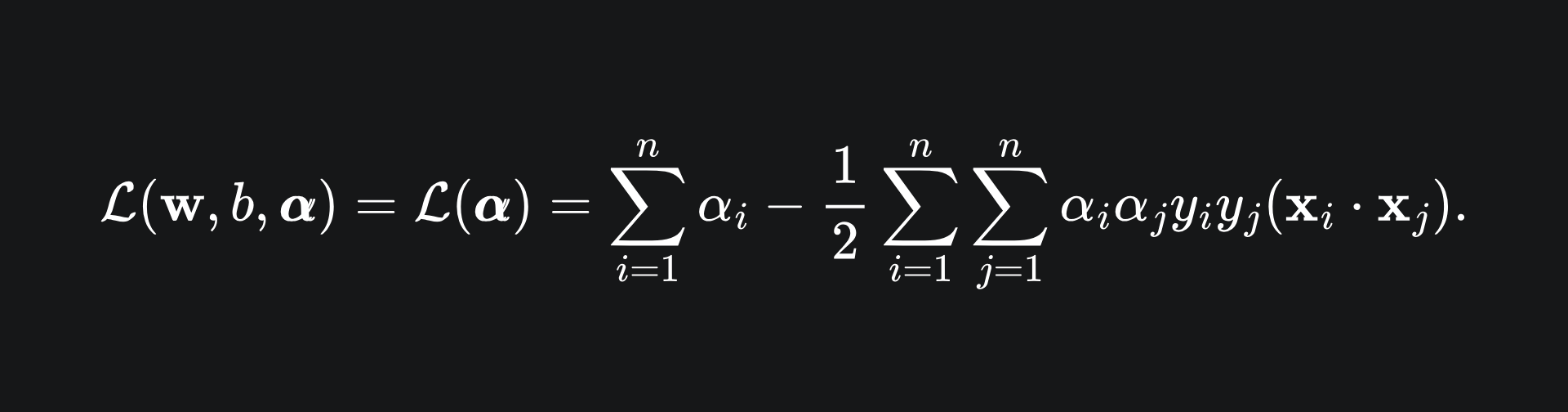
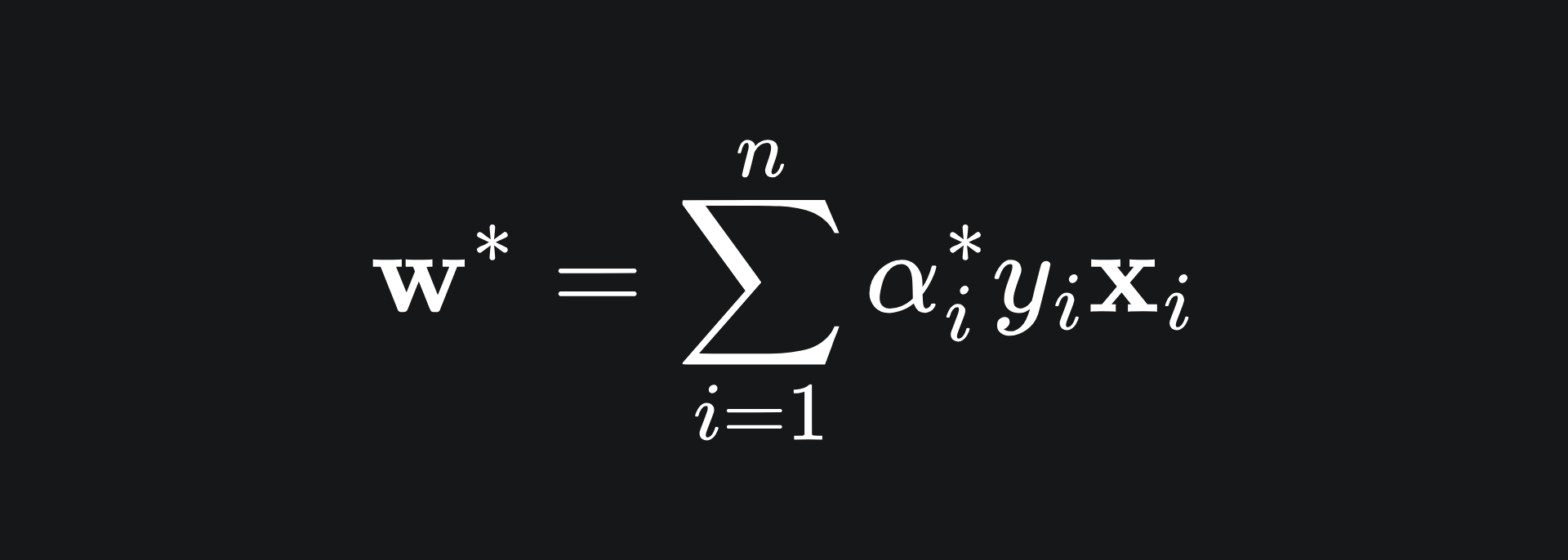
Finally, you can differentiate the Lagrangian with respect to α to find the optimal α* value. From here, the value of w* can hopefully be found³. Namely,

\(\textbf w^* = \sum_{i=1}^n\alpha_i^*y_i \textbf x_i\)

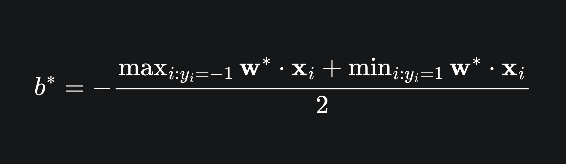
Finally, we need b*. This value represents the intercept of the decision boundary, which we want to be midway between the w*·x + b* = +1 and w*·x + b* = -1, on which the support vectors S+ and S- lie respectively. We can capture all of this is one equation:

\(b^* = - \frac{\max_{i : y_i=-1} \textbf w^*\cdot\textbf x_i + \min_{i : y_i=1} \textbf w^*\cdot\textbf x_i}{2}\)

🚨 Very important insight 🚨

Crucially, the solution for the Lagrangian (and in turn the whole SVM) depends on the dot products between the data points {x_1,…,x_n}. This is the main reason why we solved our SVM problem using the dual problem rather than the primal version. We shall revisit this dot product dependence next week!

Packing it all up

This week’s article was quite the foray into the maths of machine learning, but it’s a necessarily evil to help us with the final article on SVM next week⁴! Hope you’re not sick of the SVM yet. Either way, let me know in the comments.

Before that though, here’s a summary of this article:

• Constrained optimisation problems, such as that of our SVM problem, can potentially be explicitly solved using the method of Lagrange multipliers.

• Constrained optimisation problems can be formulated into the so-called primal problem and dual problem. Under certain conditions, the solutions to these problems coincide.

• For the SVM, the dual problem leads us to a solution which depends on the dot product between data points. We will see how useful this is next week! (Spoilers: it’s extremely useful.)

Training complete!

I really hope you enjoyed reading!

Do leave a comment if you’re unsure about anything, if you think I’ve made a mistake somewhere, or if you have a suggestion for what we should learn about next 😎

Until next Sunday,

Ameer

PS… like what you read? If so, feel free to subscribe so that you’re notified about future newsletter releases:

Sources

• Lecture notes from Stanford’s CS229 Machine Learning course (check out chapter 6): https://cs229.stanford.edu/main_notes.pdf

• Slides on convex optimisation from NYU: https://davidrosenberg.github.io/mlcourse/Archive/2017/Lectures/4a.convex-optimization.pdf

• In full generality, the optimal value for the dual problem is a lower bound for the optimal value of the primal problem, i.e. d* <= p*. But under certain conditions, the gap between the two values can be reduced to zero (so-called ‘zero duality gap’). Check out these Stanford lecture notes on Lagrangian duality (note that I don’t agree with the title!): https://cs.stanford.edu/people/davidknowles/lagrangian_duality.pdf

• The following online page from Cornell Tech contains some information on Sequential Minimal Optimisation, which can be used to find w* once we have found α*: https://kuleshov-group.github.io/aml-book/contents/lecture13-svm-dual.html

1. The sources I have referenced at the end of this article will provide more context, so do check them out if you’re curious. But yeah, kinda impossible to cover everything in one article, apologies.

2. Check out the ‘Sources’ section at the end of the article for more information.

3. This relies on a technique called Quadratic Programming. The most common form to solve the SVM problem is the Sequential Minimal Optimisation algorithm (check sources).

4. Or at least, I think we’ll be wrapping up the SVM next week 👉🏼👈🏼 I plan on discussing whether the SVM can handle linearly inseparable data. Certified banger incoming.