
How is reverse mode automatic differentiation suited to neural networks?
Exploring the relationship between forward/reverse automatic differentiation and the Jacobian matrix.

Hello fellow machine learners,
Firstly, a big thanks is in order to you all, the readers- we surpassed 500 subscribers this past week! I started writing this newsletter in December 2024, and am grateful for the support across that time. Hopefully the posts have been informative and fun to peruse. As always, let me know in the comments (or by DM) of any machine learning topics you want covered in the future :)
Last week, we discussed a few methods of differentiating functions, concluding the conversation with forward mode automatic differentiation. Forward mode is better than numerical and symbolic differentiation, because it tracks both the values and the gradients of the constituents of the function, which is more computationally efficient. We also described an issue with forward mode that will be elaborated on more in the next section.

I would strongly recommend you have a read of that article before continuing with this one…
👉🏼👈🏼 I’ll wait 👉🏼👈🏼
…all done? Nice- then let’s get to unpacking!
The Jacobian
Let’s begin with some mathematical theory. Last time, we touched on scalar-valued functions, which take the form
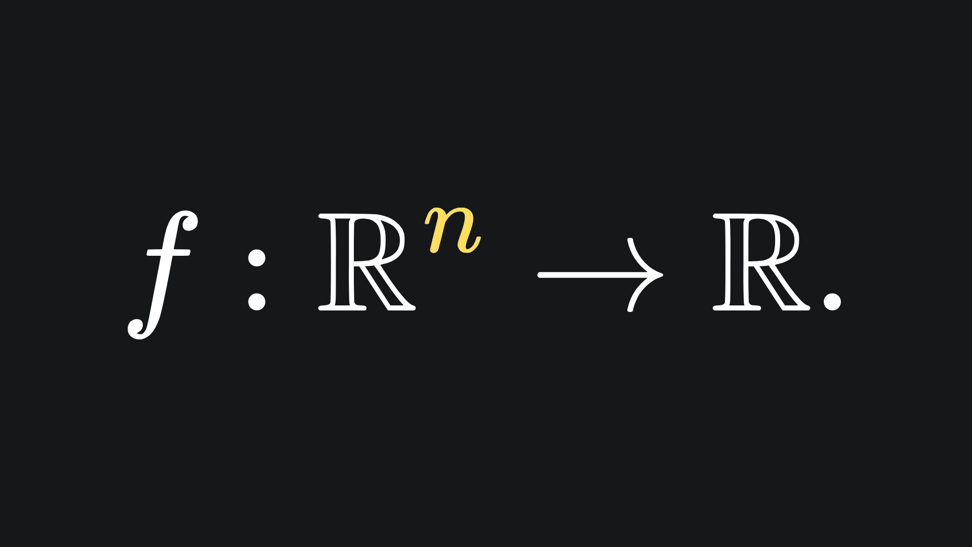
What is the derivative of this function? Well, since there are n distinct inputs, we ought to get n distinct derivatives. In particular, we get n partial derivatives, which can be aligned nice and neatly in a column:
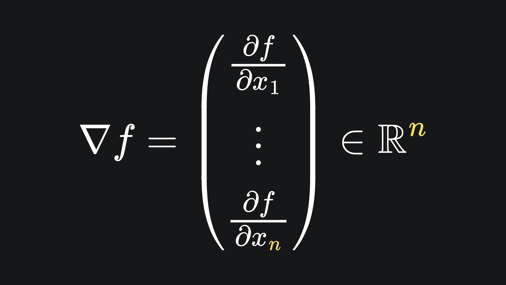
And to evaluate the derivative of f at a vector x, we simply plug the components of x into the gradient vector. (This tells us what direction we should move from the point x in order to increase the value of f as much as possible.)
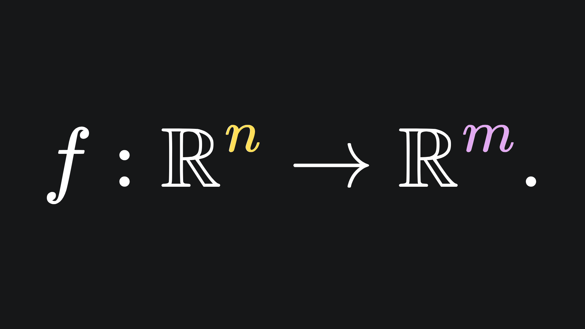
But what if f is instead a vector valued function? I.e. it takes the form
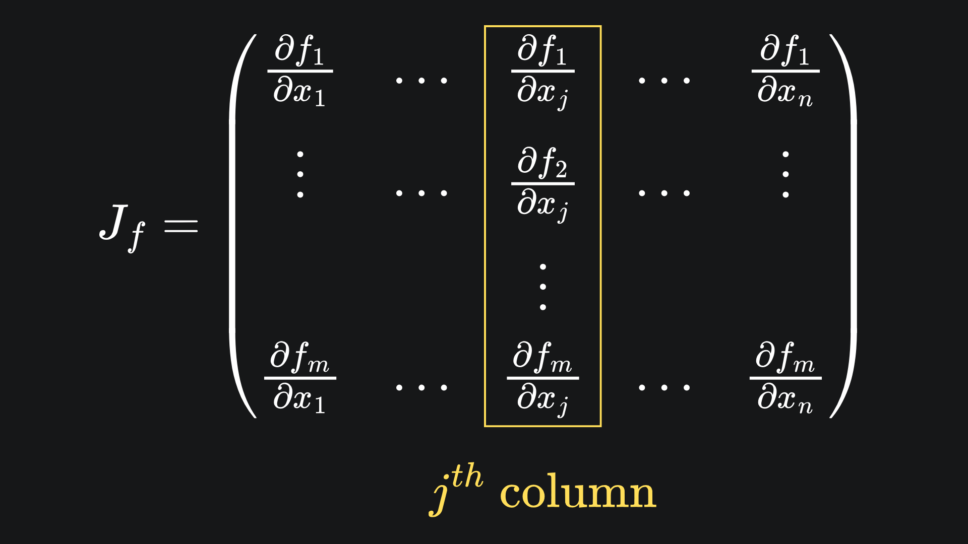
In this case, we get n partial derivatives for each of the m outputs. This yields nxm partial derivatives in total. In particular, we can arrange the partial derivatives for each output variable in their own column, transpose to get a row, and then stitch the rows together to form a matrix. The result is the Jacobian matrix of the function f:
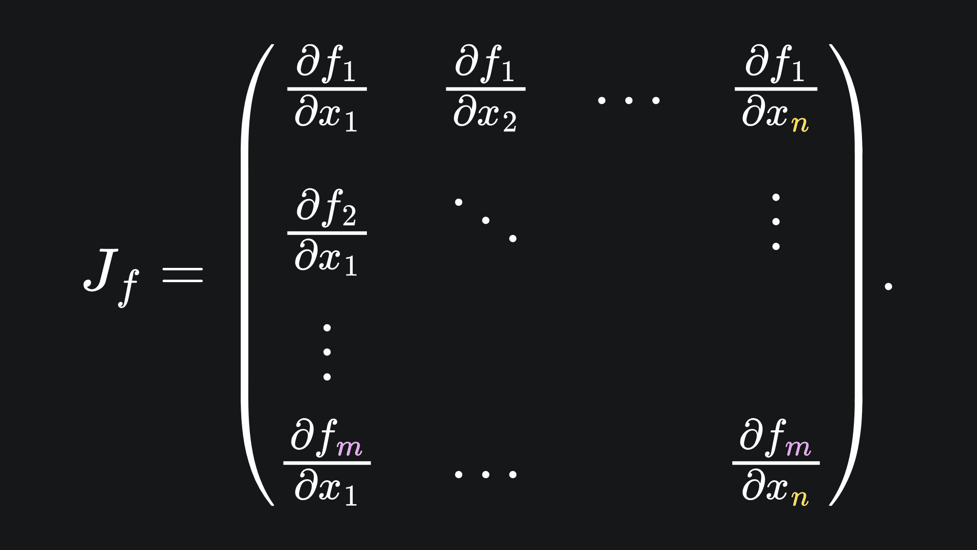
When evaluated at a vector x, the Jacobian is the matrix that provides the best linear approximation of f at x. And in neural networks, the partial derivatives are precisely what we wish to evaluate, for use within a gradient descent technique.
Connection to forward mode automatic differentiation
We can actually evaluate the columns of the Jacobian of a function using forward mode AD! This was alluded to last week, we just didn’t reference the Jacobian back then. Recall the function
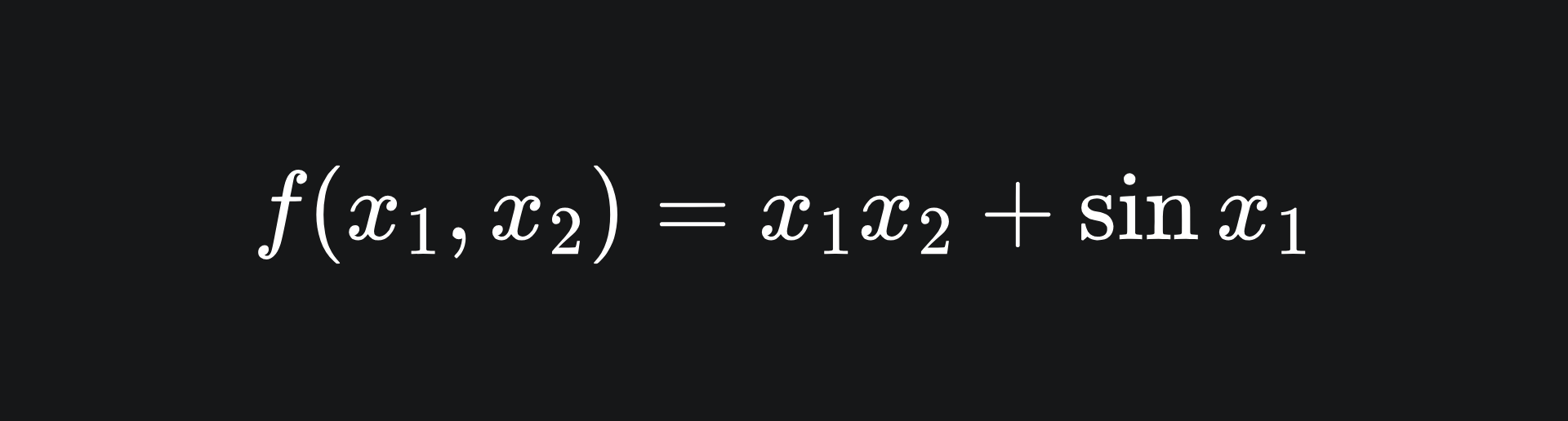
with input, intermediary and output variables
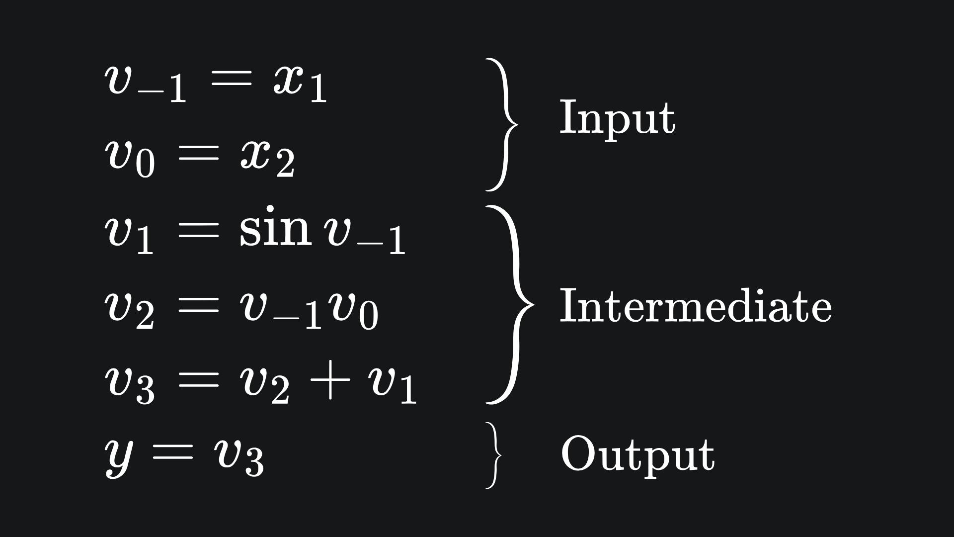
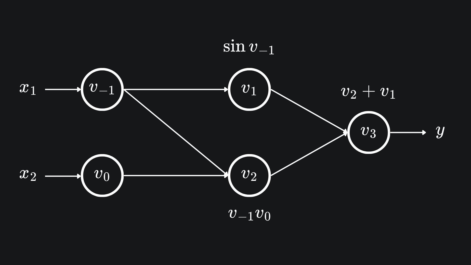
represented visually with the following computational graph:
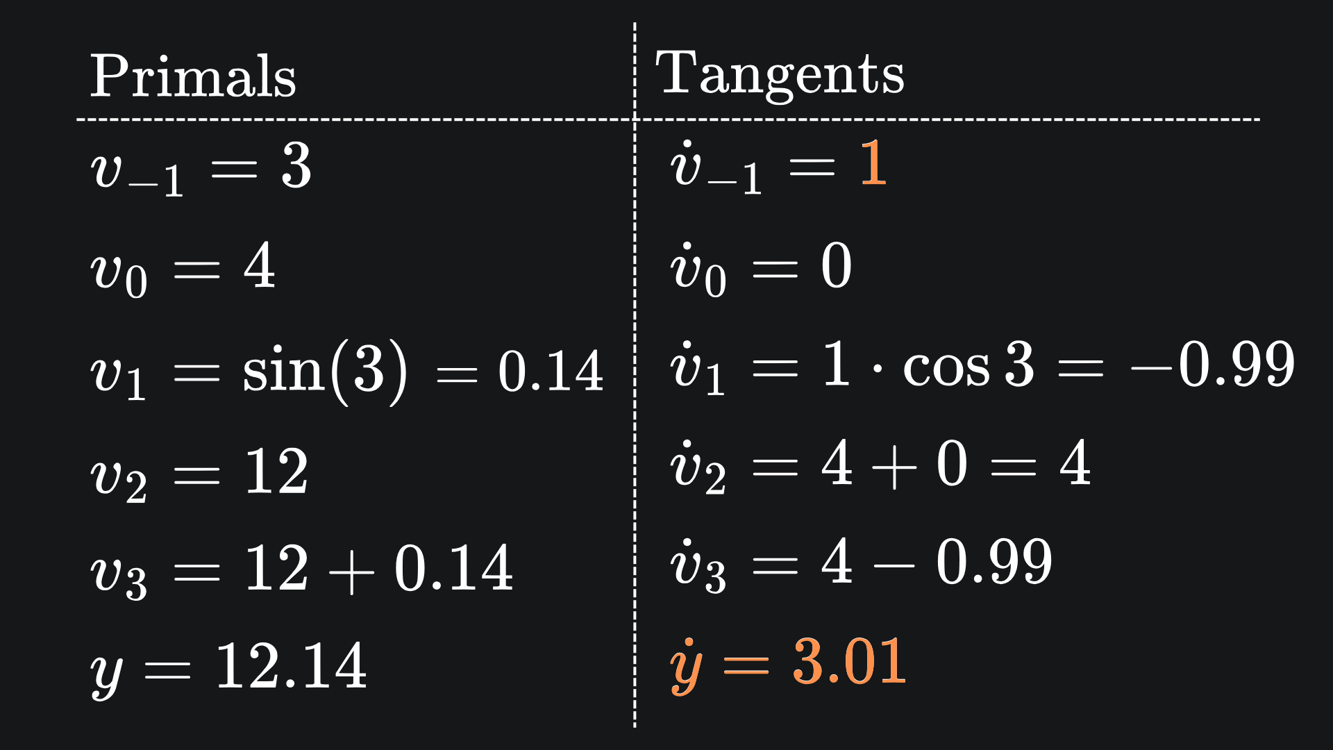
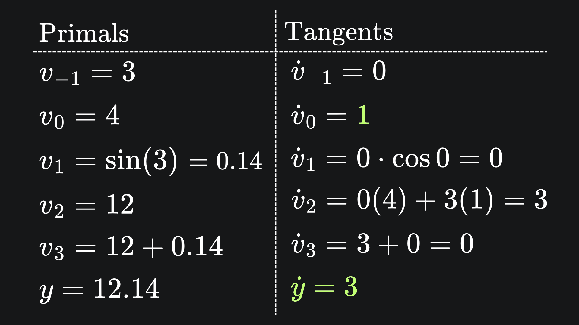
We used forward mode to evaluate ∂f/∂x1 at the point (x1,x2)=(3,4). In the end, we got the value 3.01 (to 2dp) by using the forward mode primals-tangents table with:
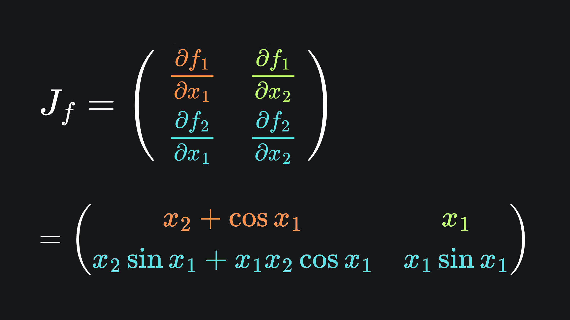
Let’s verify that this is consistent with the Jacobian of f. Applying our usual calculus rules, the explicit form of the Jacobian looks like:
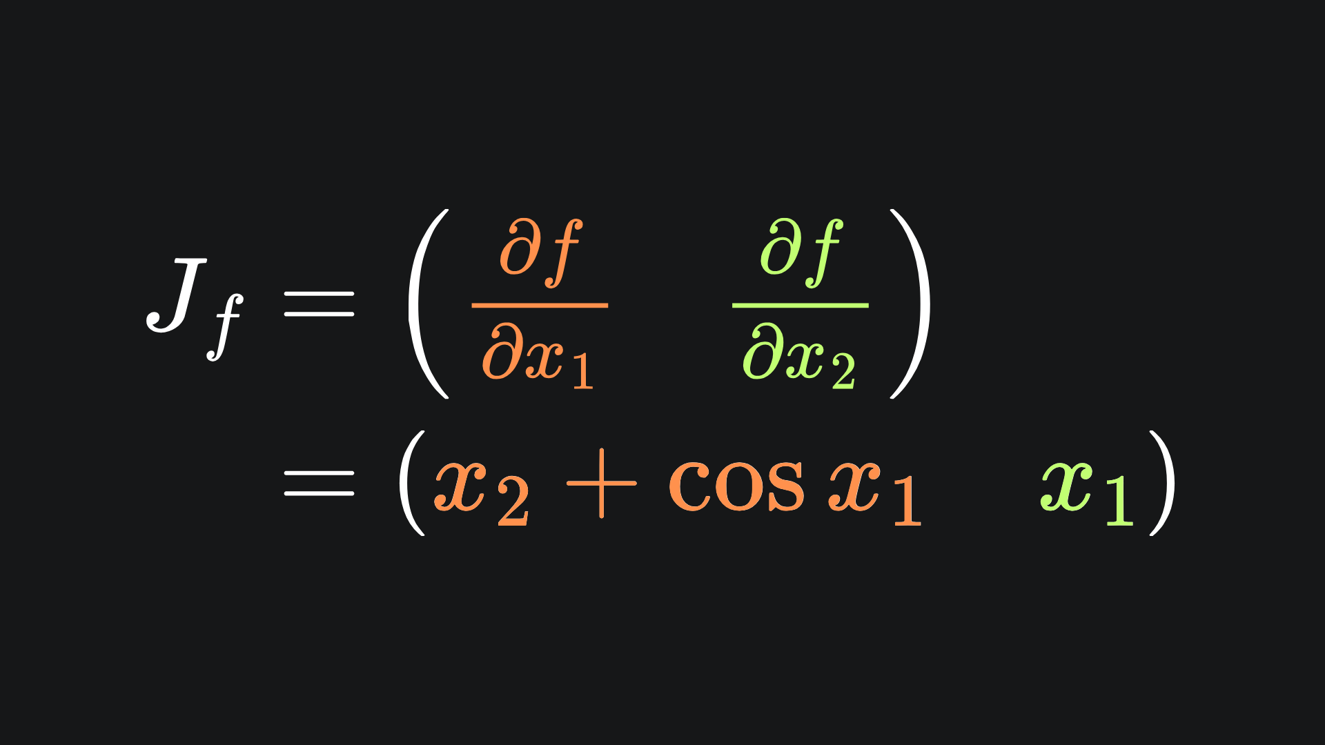
Since f is scalar-valued, the Jacobian matrix is just a single row. If we plug in (x1,x2)=(3,4), we end up with:
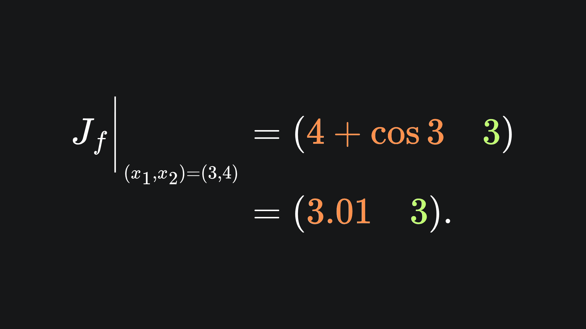
And indeed, the value in orange is precisely what last week’s forward mode pass resulted in. Awesome 😎
Downsides
This allows us to compute the partial derivatives of all the output variables with respect to a single input variable. That’s great, but it means that, if we want partial derivatives with respect to some other input variable, we have to run the entire forward mode process again. For the above example, if we wanted ∂f/∂x2 instead, then we’d need to flip the values for the first two tangents and feed in all the forward pass values. This is shown below:
(The value is green is precisely what we got when computing the Jacobian explicitly. No surprises there.)
Computing this new forward pass didn’t take too long for this toy example. But what if our function represents a neural network, a structure in which the input dimension n is usually far larger than the output dimension m? Cast your mind back to this example:
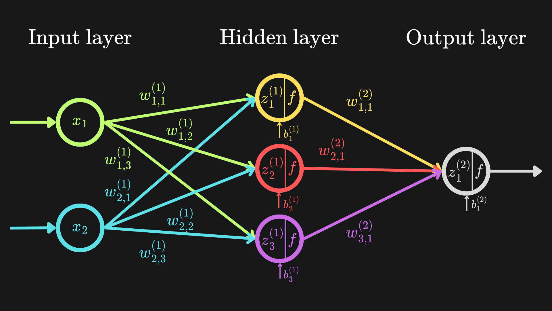
Recall that a neural network is parametrised by its weights and biases. This means that this network is akin to a function of just one output, but thirteen inputs. The Jacobian for this neural network would be a 1x13 matrix. So if we wanted all thirteen partial derivatives (i.e. for use in gradient descent), then we would have to use forward mode AD thirteen times.
Yikes. Looks like this doesn’t scale well at all…
Reverse mode automatic differentiation
We now introduce a different version of AD that’s better suited to our neural network needs.
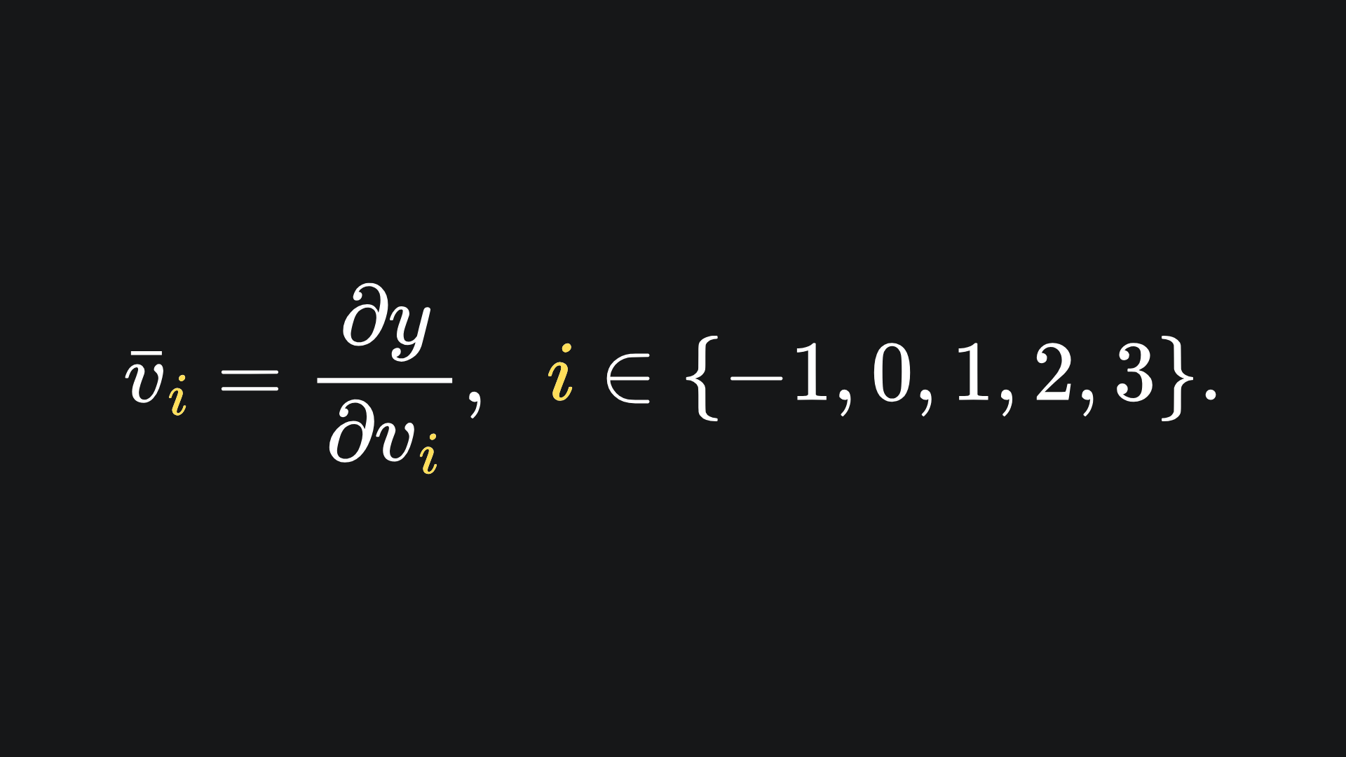
With forward mode AD, we tracked the tangents of the intermediary variables. This time, however, we’re going to track the adjoints, which are the partial derivatives of the chosen output dimension with respect to each intermediary variable. Let’s use last week’s example to illustrate how this may work in practice. The function from before is
and has adjoints defined as
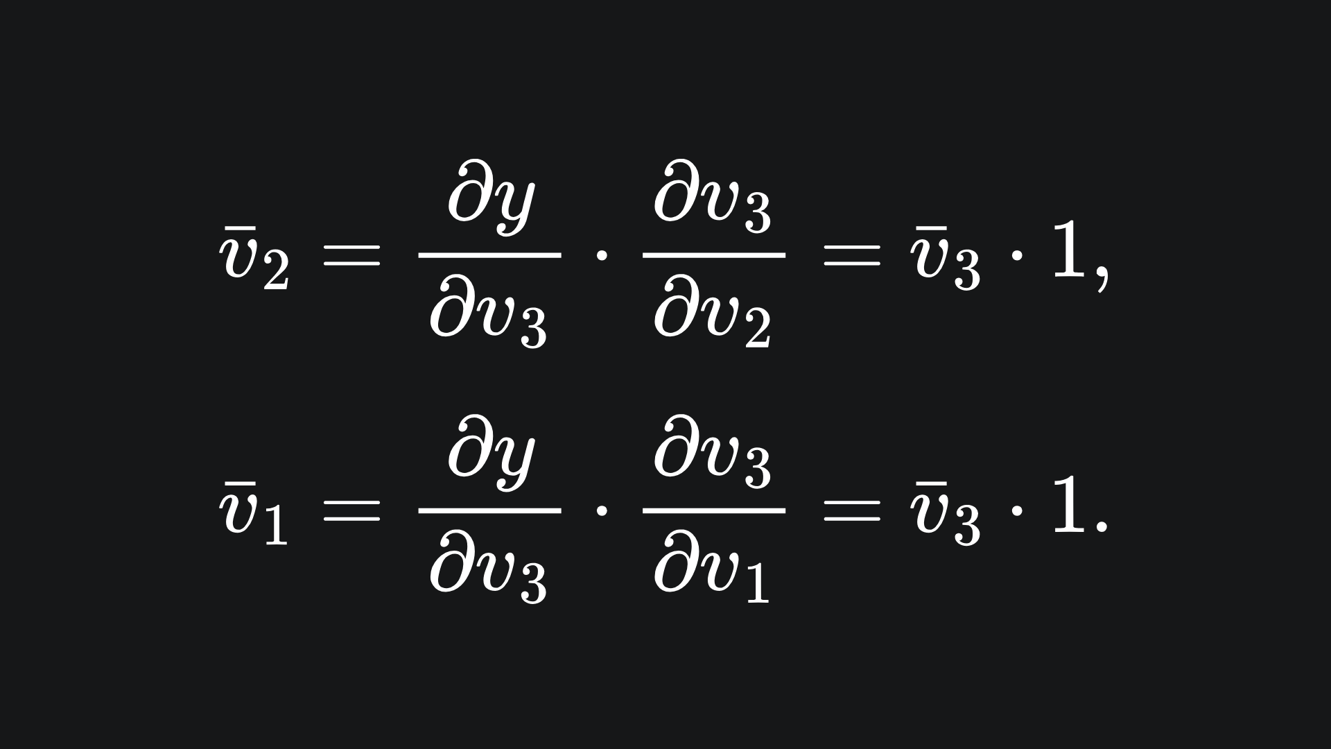
The computation of primals is the exact same as before. As for adjoints, we start with the desired output dimension (in this case we only have one output dimension, y). From here, we compute the partial derivatives of this output variable with respect to all the intermediary variables. We start with the adjoint of v3, because it relies directly on y, and the adjoints of the other intermediary variables rely on the adjoint of v3. This first one is simple:

For the next two adjoints, we must invoke the chain rule:
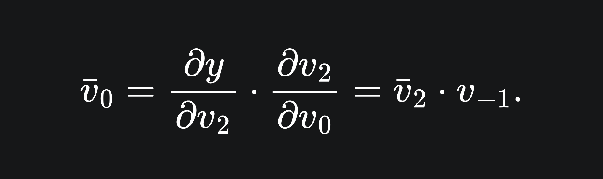
The adjoint for v0 follows similarly:
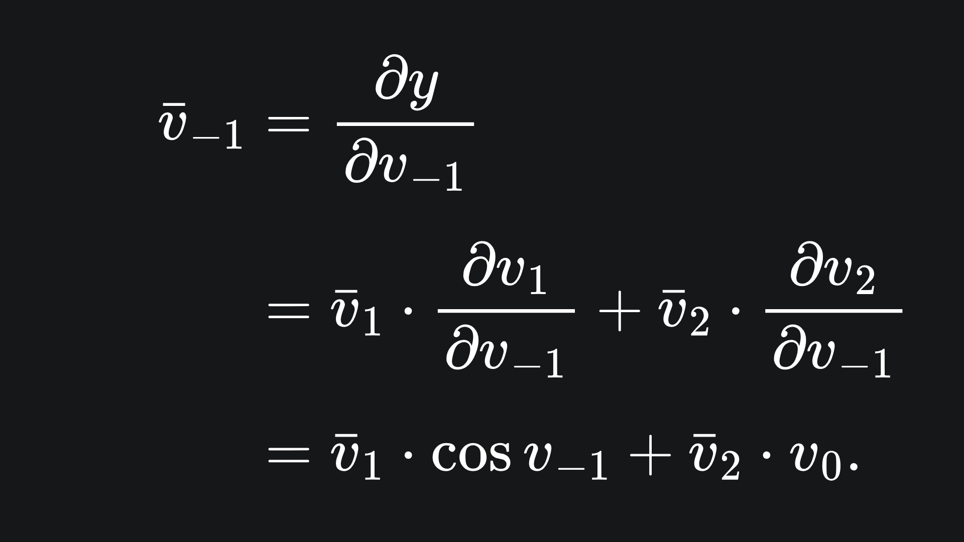
However, v-1 is slightly different, because it depends on both v1 and v2, meaning that ∂y/∂v-1 depends on ∂y/∂v1 and ∂y/∂v2. This means we must apply the law of the total derivative:
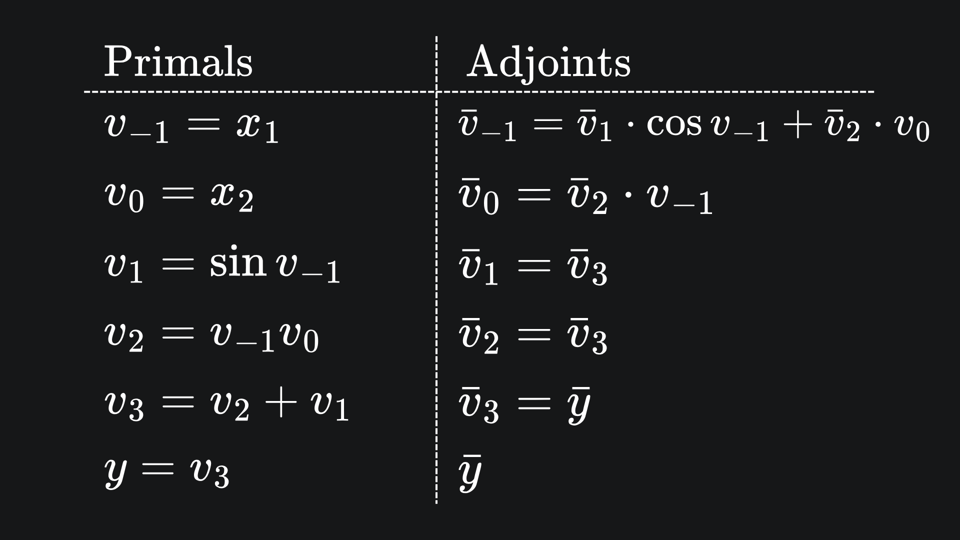
We can present this all nice and neat in a table of primals and adjoints:
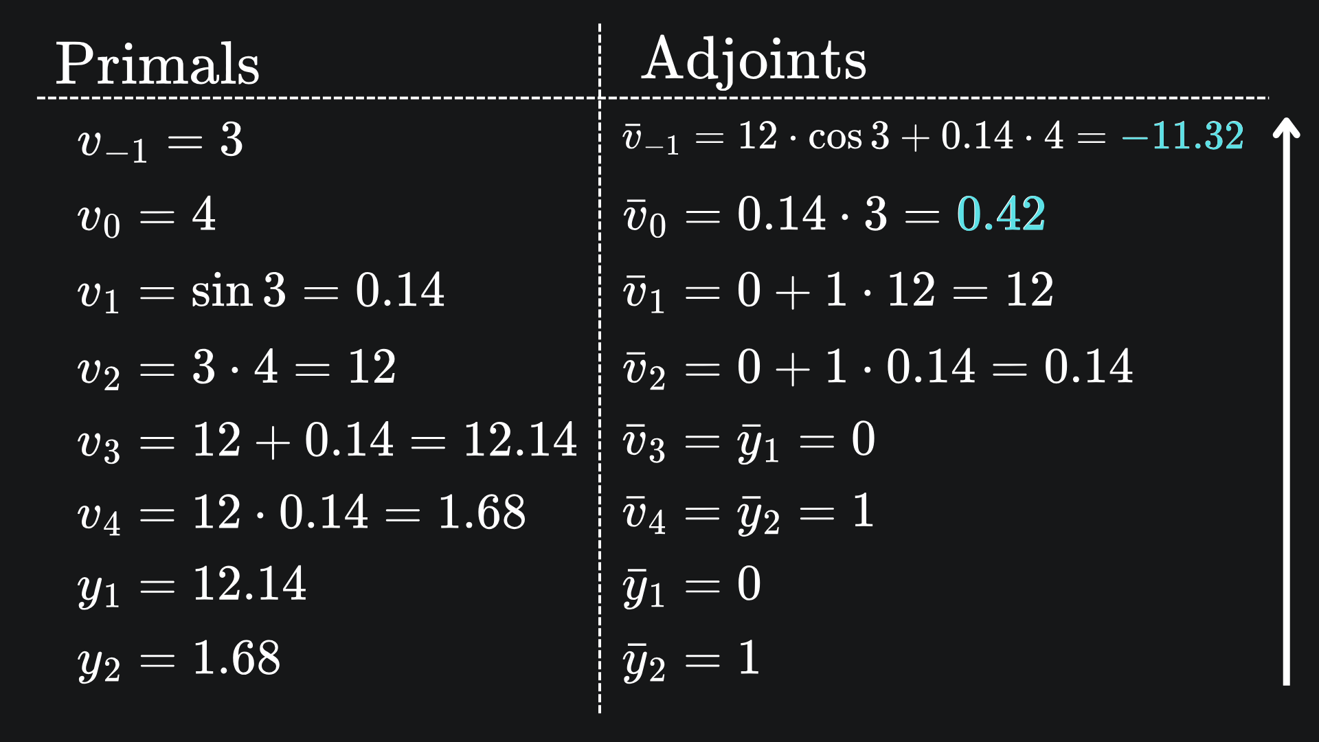
Now to substitute in the numbers! If we want the partial derivative of y with respect to each input variable, again evaluated at (x1,x2)=(3,4), we start by setting the adjoint of y equal to 1, and following the numbers through from the bottom to the top:
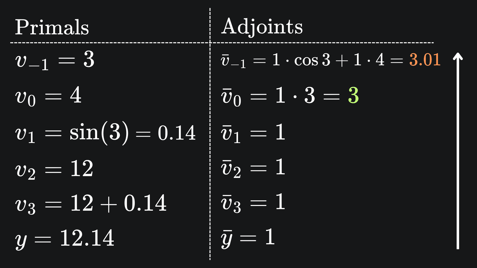
This process is called reverse mode automatic differentiation. No awards for guessing why it’s called that.
Notice that, through a single reverse mode pass, we naturally recover both ∂f/∂x1 and ∂f/∂x2. In fact, for a scalar-valued function of n input variables, one reverse mode pass gives us all the partial derivatives!
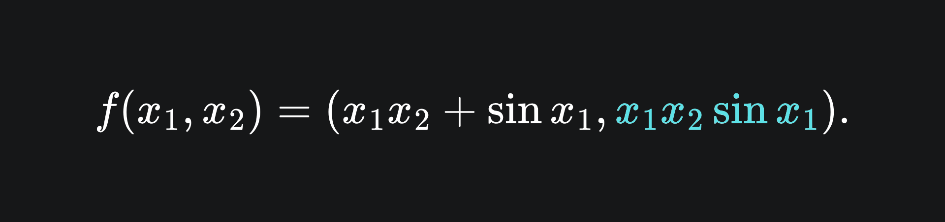
What about if f has two output dimensions? The example we used last week was
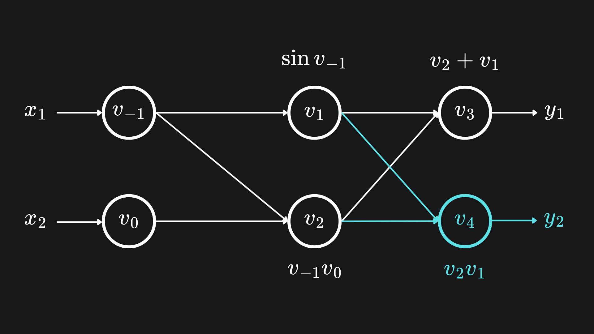
The extension to the computational graph looked like
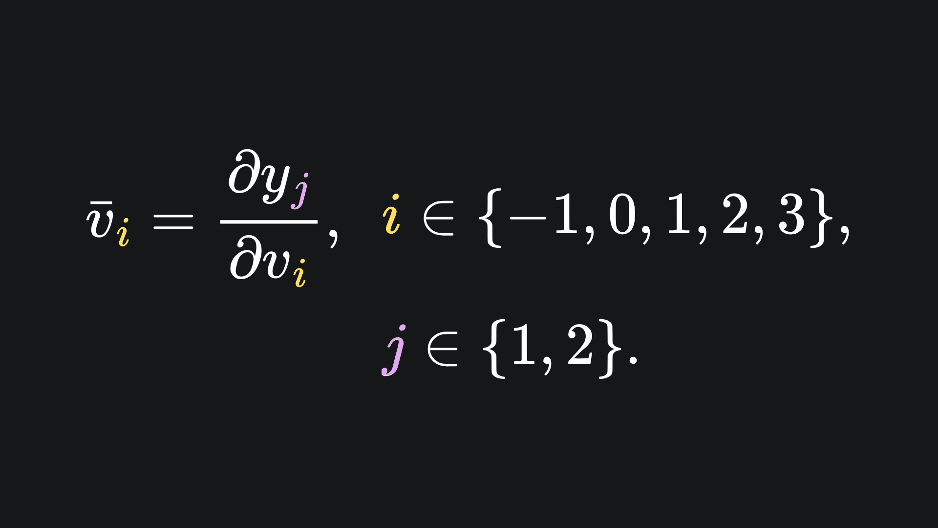
In this case, our definition of adjoints should now include a subscript for the output variables:
and we can update our table of adjoints as follows:
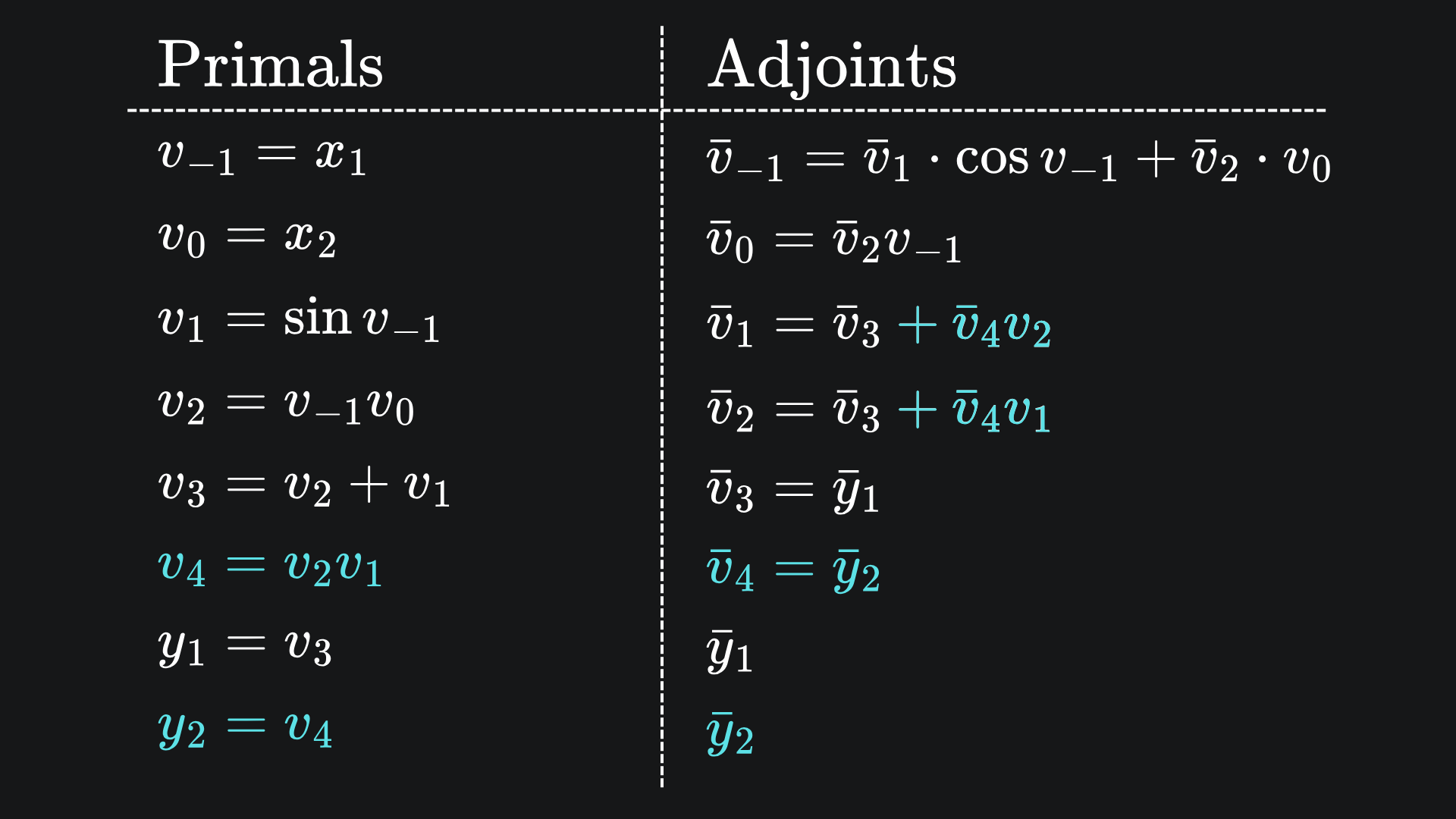
The intermediary variables v1 and v2 now feed into v4 as well as v3, so we have to apply the law of the total derivative to their adjoints, hence the modification in blue.
Since f is now vector-valued, the Jacobian matrix for f gets a new row:
Suppose we wanted to evalutate both ∂f1/∂x1 and ∂f1/∂x2 at the point (3,4). Let’s show that one reverse pass is all we need:
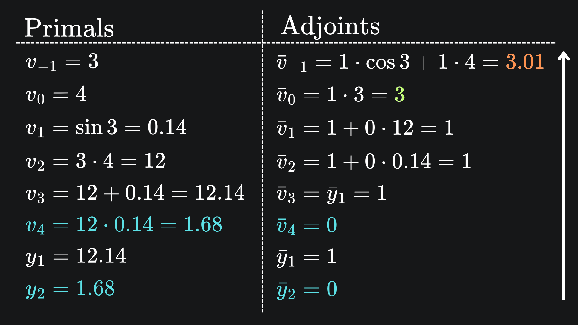
We’re greeted with our familiar 3.01 and 3 😎
To get the partials ∂f2/∂x1 and ∂f2/∂x2, we set the adjoint of y1 to 0 and the adjoint of y2 to 1. This demands a separate reverse pass compared to acquiring ∂f1/∂x1 and ∂f1/∂x2.
Here is what that looks like in the primals-adjoints table (2dp as always):
I will leave you to verify that these derivatives coincide with the second row of the 2x2 Jacobian.
So if f is vector valued, then one reverse mode pass gives us the partial derivatives for just one output variable, but with respect to all input variables.
Connection between forward mode and reverse mode
This is probably a good time to take stock of our two modes within the context of an arbitrary vector-valued function f of n input variables and m output variables.
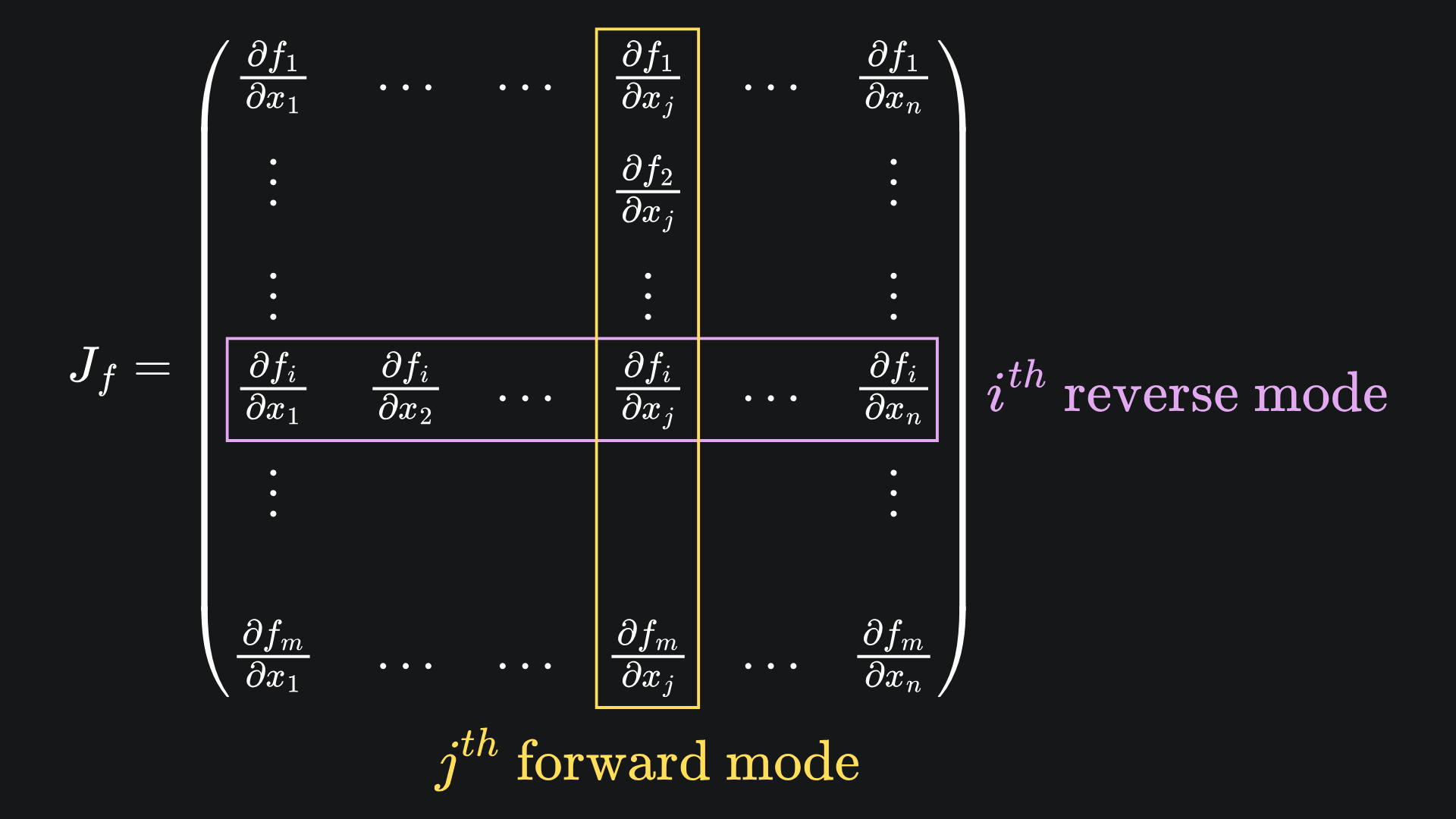
For a fixed input dimension j, forward mode AD yields the partial derivatives of all the output dimensions with respect to input j. This corresponds to the j-th column of the Jacobian matrix for f:
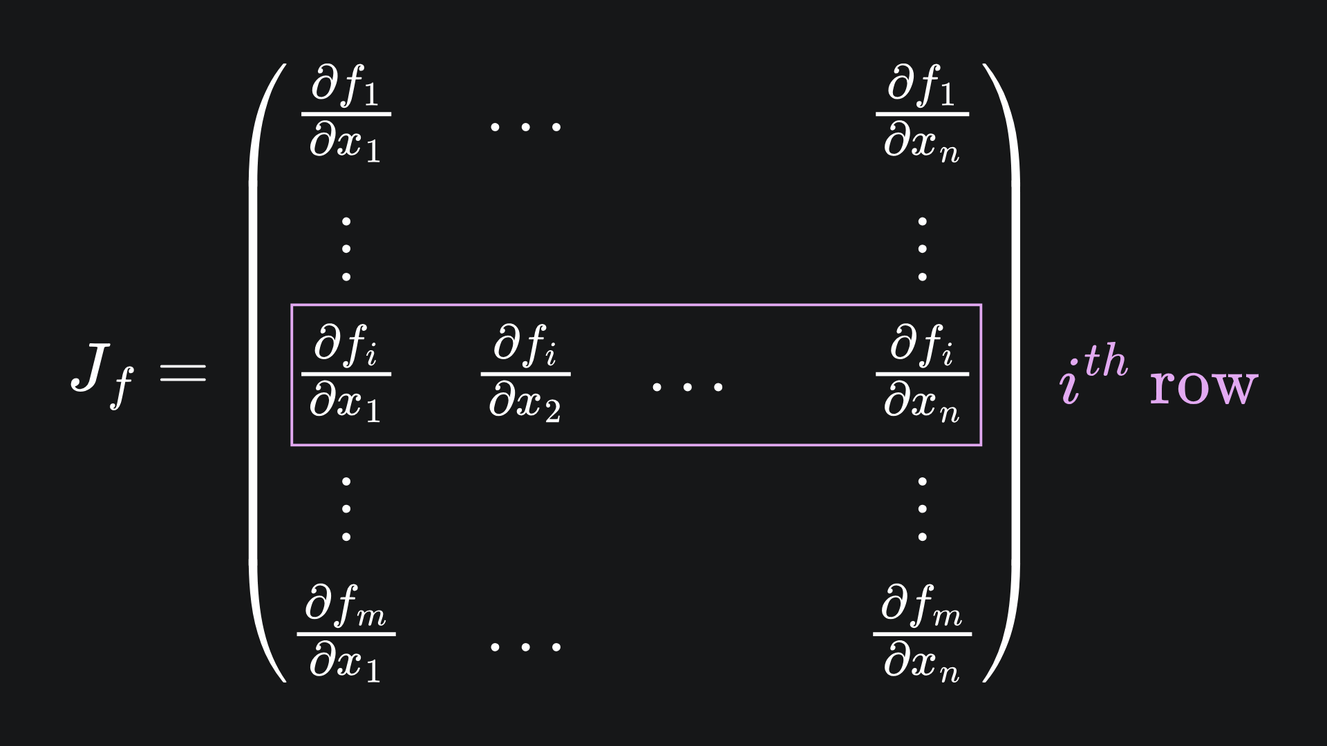
Conversely, for a fixed output dimension i, reverse mode AD yields the partial derivative of i with respect to all input dimensions. This corresponds to the i-th row of the Jacobian of f:
Don’t forget the main question we’re trying to answer: why is reverse mode AD better suited to neural networks? Well, the function represented by a neural net will consist of far more inputs than outputs, i.e. the corresponding Jacobian will have far more rows than columns. In such cases, reverse mode is more efficient for helping us recover all the entries of the Jacobian.
Packing it all up
Here is a nice visual summary of what’s been discussed today:
And it wouldn’t be a “Packing it all up” section without some package emojis and summaries:
📦 The Jacobian matrix of a vector-valued function f stores all the partial derivatives of f. The (i,j)-th entry of the Jacobian corresponds to the partial derivative of the i-th output with respect to the j-th input.
📦 Each pass of forward mode automatic differentiation recovers a column of the Jacobian. Conversely, each pass of reverse mode yields a row. We can choose which column or row we want by modifying the values of the tangents or adjoints respectively.
📦 Reverse mode automatic differentiation is well-suited to neural networks. This is because we can think of neural network as a function with weights/biases as input dimensions. In this case, there are often far more input variables than output variables. And in such a case, reverse mode requires fewer passes to recover the full Jacobian compared to forward mode.
Training complete!
I hope you enjoyed reading as much as I enjoyed writing 😁
Do leave a comment if you’re unsure about anything, if you think I’ve made a mistake somewhere, or if you have a suggestion for what we should learn about next 😎
Until next Sunday,
Ameer
PS… like what you read? If so, feel free to subscribe so that you’re notified about future newsletter releases:
Sources
My GitHub repo where you can find the code for the entire newsletter series: https://github.com/AmeerAliSaleem/machine-learning-algorithms-unpacked
Here is an excellent blog on the same topic that I found on HuggingFace