
Gradient boosted trees: an intro to boosting ensembles 🚀
Explaining how gradient boosting iteratively corrects errors to build a powerful ensemble.

Hello fellow machine learners,
Last week, we discussed the random forest, an ensemble method which aims to reduce the variance of any constituent tree through the bagging procedure.
This time, we will discuss a very different tree-based algorithm that also promises to outperform a single decision tree: namely, the gradient boosted algorithm.
We will first describe the steps of the algorithm and then explain why it actually works.
Let’s get to unpacking!
The gradient boosting process
The main idea behind the gradient boosting algorithm is to sum together a sequence of ‘weak learner’ models, with the aim of reducing the errors incurred by each previous sum of models. By ‘weak learner’, we are referring to ML models that are slightly better than random guessing- but we’ll explore this a bit more later.
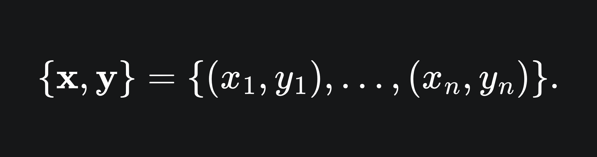
Suppose that we train an initial decision tree model, say, F1, on the dataset
The error made by the model can be quantified by a loss function. A loss function is a function that quantifies how badly the model has performed in learning the data, i.e. the larger the value, the worse the model has performed. For example, take a look at the mean squared error1 that’s used for regression trees:
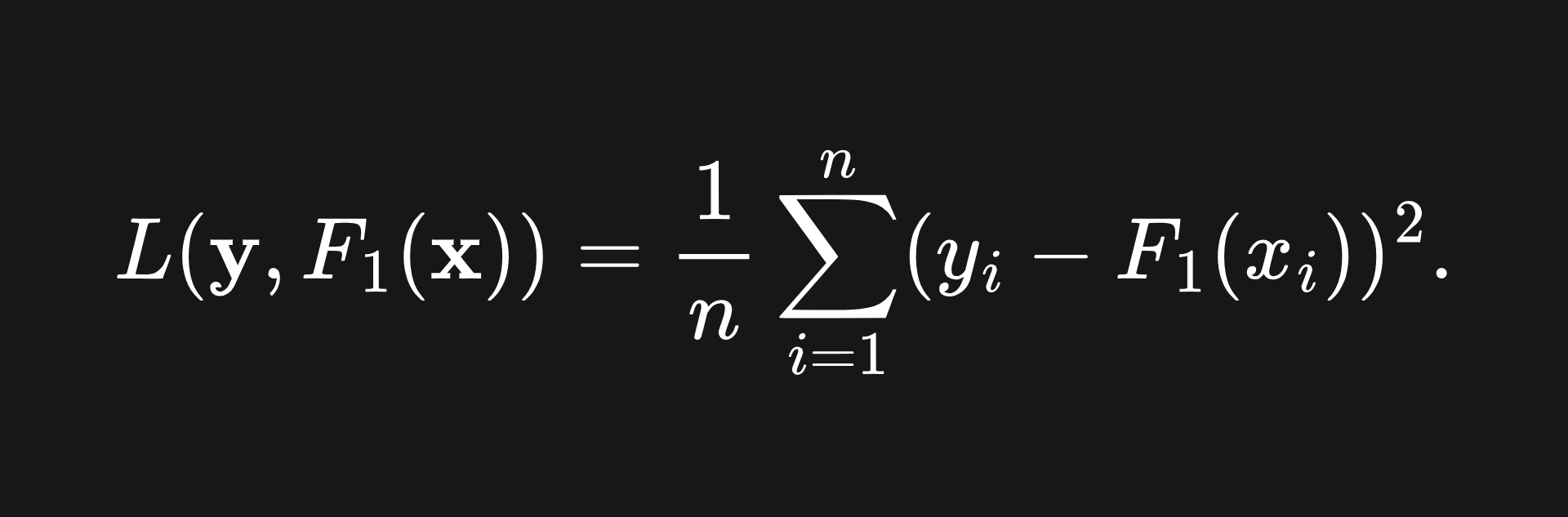
The value of this function is minimised precisely if F1 matches the data perfectly, in which case F1(xi)=yi for all i, meaning that L=0. Otherwise, the value of L will be greater than zero.
Our aim is to minimise the loss incurred by the learner F1. To do this, we compute the negative gradient of the loss function with respect to all the predictions on the training data made by F1:

This yields a set of n values. Next, we train a new weak learner, let’s call it f2, on these values:
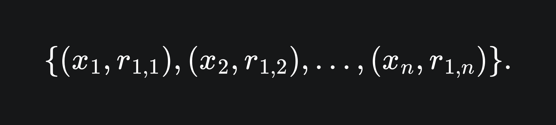
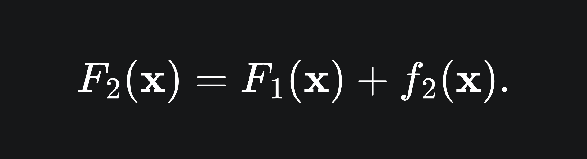
So the hope is that f2(xi)≈r1,i for all i. The point of this is that f2 will help to adjust the errors of F1. At this stage, we could set our next model in the ensemble to be the sum of our two current models:
However, we want to be careful about how much of f2 we incorporate. This is because adding too much of f2 can result in an ‘over-correction’- we’ll come back to this in a bit.
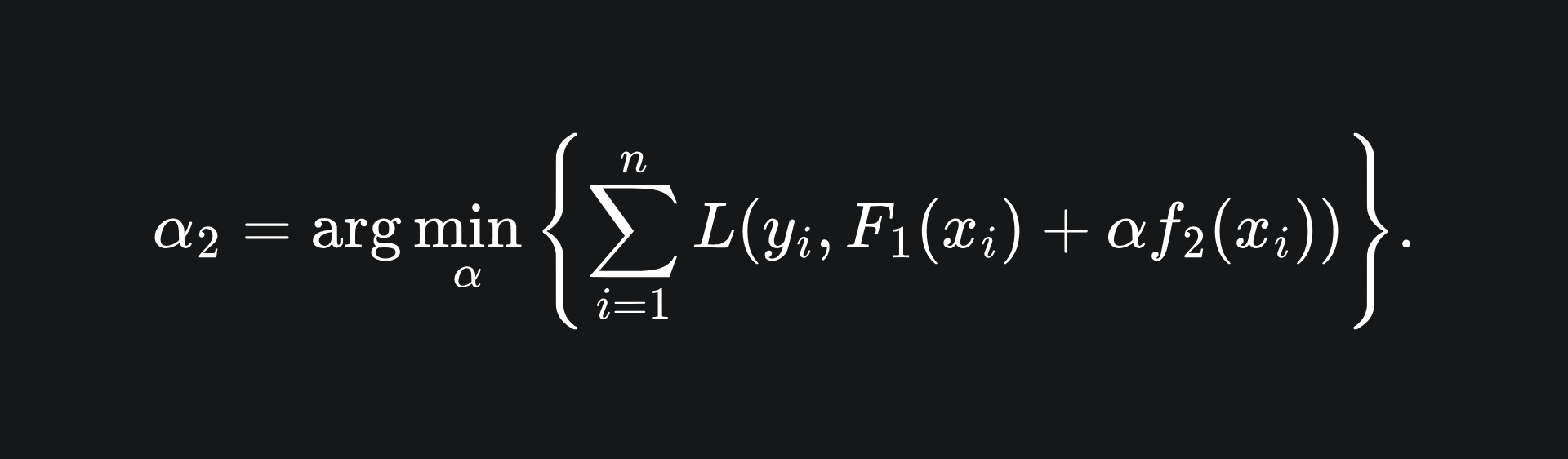
By introducing a ‘learning rate’ α, we can control the contribution of f2 to the overall ensemble. We can tune the value of α in accordance to the learning rate value that minimises the loss across all the training data:
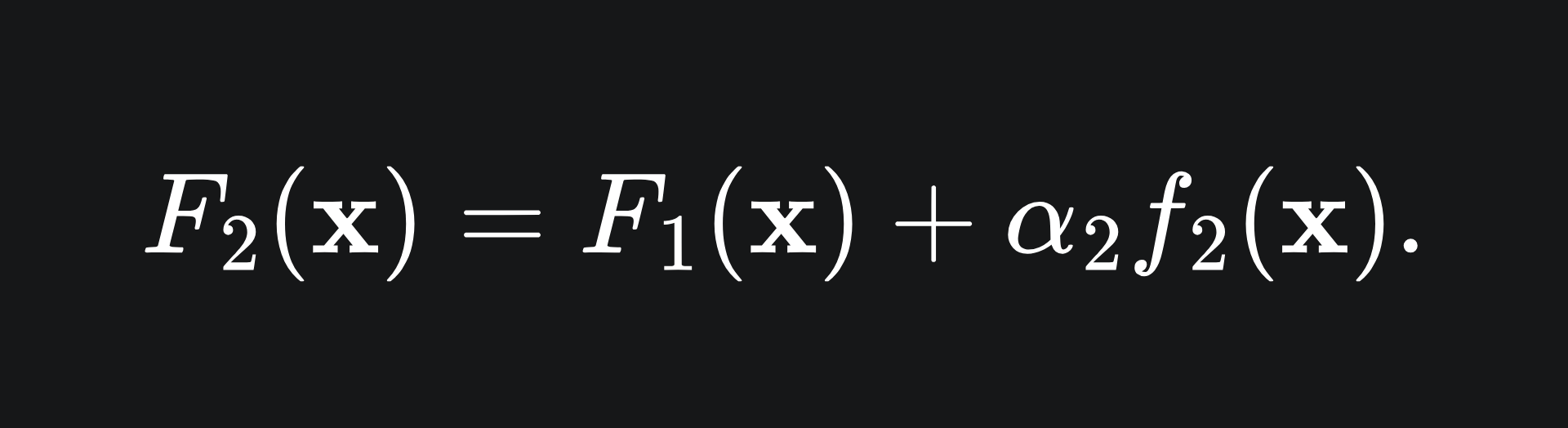
Now, the second model in our ensemble takes the form
At this stage, we repeat the procedure to add as many weak learners to the ensemble as possible, e.g. in order to find F3, we:
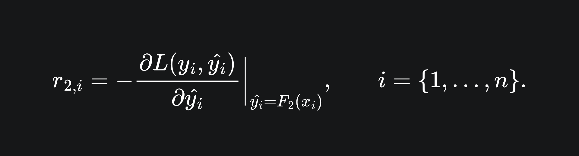
Compute the negative gradient of the error terms

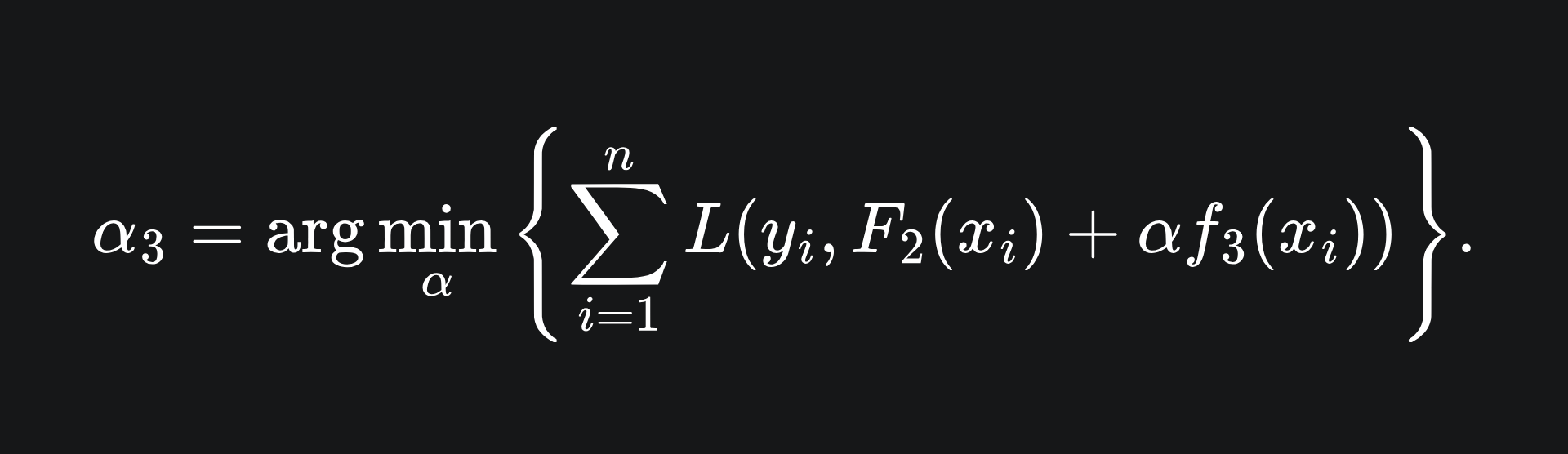
Train the model f3 on the corresponding data
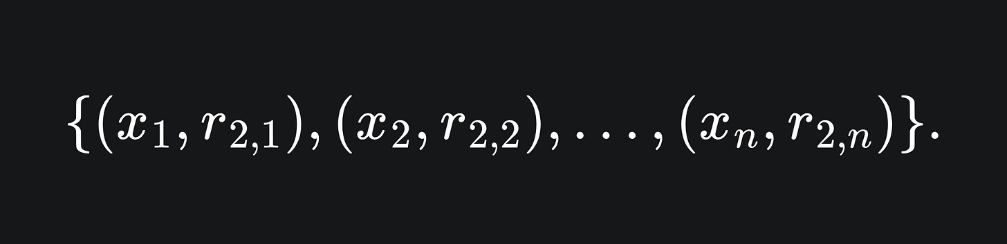
Figure out the optimal learning rate, i.e. how much of f3 to actually contribute to the ensemble:

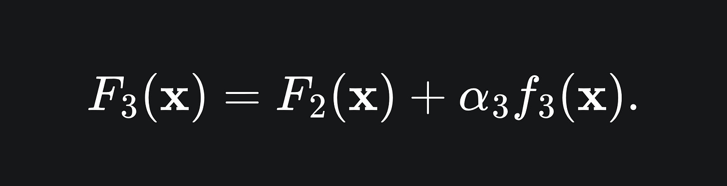
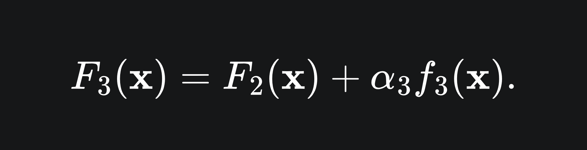
Build the next model in the ensemble:

This procedure can be extended to m weak learners in the ensemble.
Why does this work?
If we spell out what’s happening at the jth step of the algorithm, notice that

Remember that the job of learner fj is to learn the values {(x1,rj-1,1),…,(xn,rj-1,n)}. So the above can be approximated as
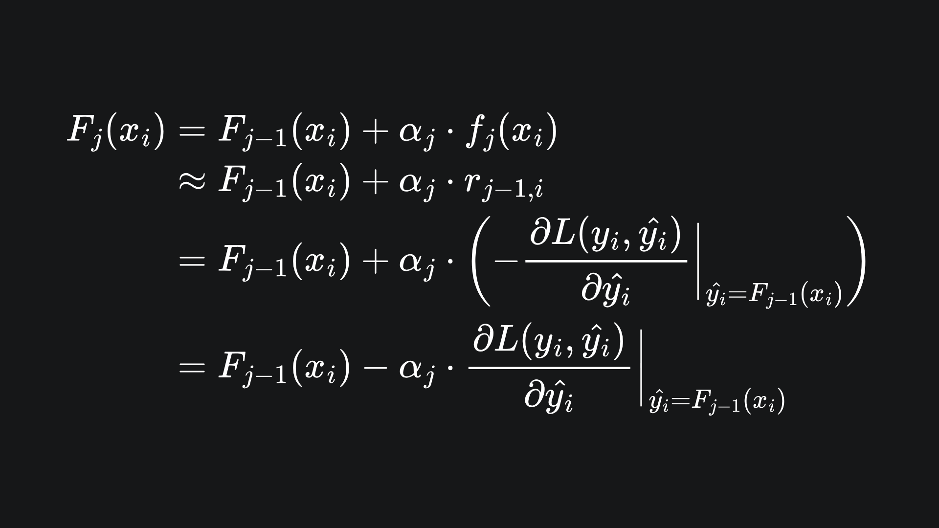
This might look quite messy, but if we focus just on the j subscripts, our algorithm is essentially
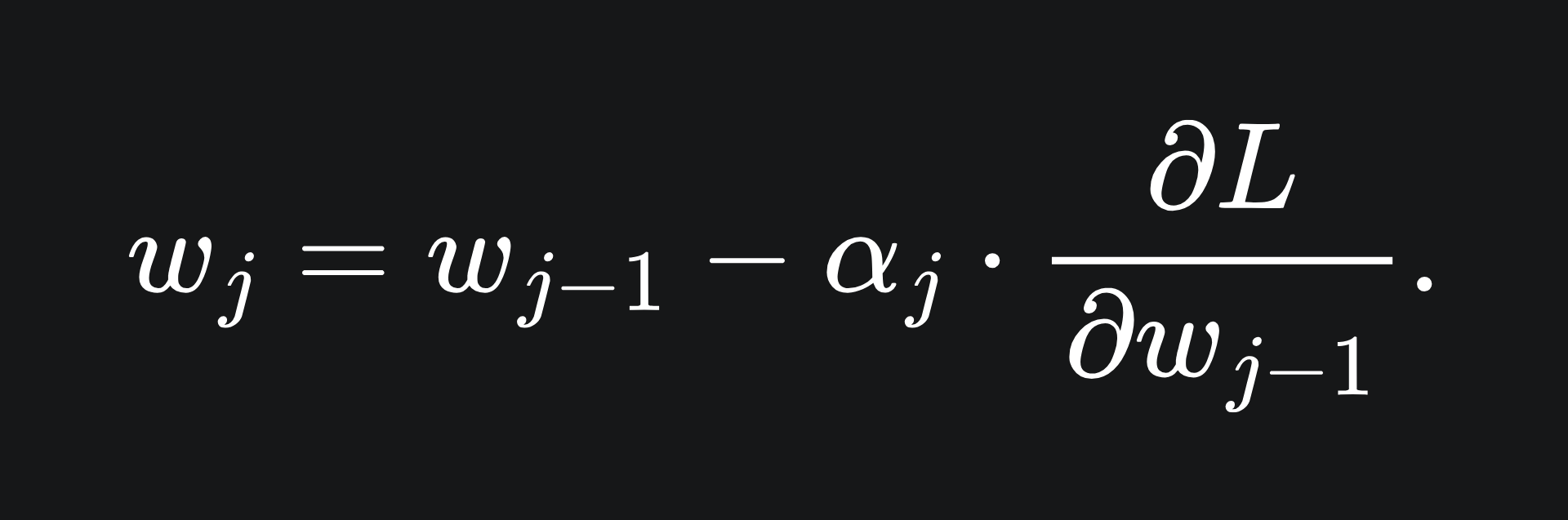
This is precisely the gradient descent algorithm!
Hopefully, this explains why we introduced the learning rate parameters αj to control the contribution of each fj. It also clarifies where the name ‘gradient boosting’ come from: we are boosting the performance of our overall model through gradient descent.
Essentially, building our boosting ensemble works to directly minimise the model’s loss! This is pretty cool in my opinion.
(Btw I am happy to write an article about gradient descent for those who aren’t familiar with it: just let me know in the comments below 😊)
Why weak learners?
The main reason is speed: it takes less processing power to train low-power models than high-power models. For example, a decision tree of depth 5 is easier to train than a decision tree of depth, say, 10, because there are fewer splitting rules for the model to learn and implement.
Gradient boosted trees
The weak learners used for gradient boosted trees tend to be decision tree stumps, i.e. decision trees consisting of a single node split. Here is an animation to depict what the boosting procedure looks like, starting from a stump and building up to a full gradient boosted tree:
Packing it all up
Another week, another ML algorithm unpacked! A lot of calculus-type ideas in this one, but it goes to showcase the utility of the gradient descent procedure, as well as the flexibility of the boosting process. Here are the key takeaways:
The gradient boosting algorithm builds up a weighted summation of weak learners in a sequential fashion.
The ensemble uses gradient descent under the hood, in order to minimise the loss of the resultant model. The learning rate is a key component of the gradient descent algorithm, which helps ensure that the steps taken to minimise the loss aren’t too large or small.
Weak learners are used as the ensemble’s constituents, because of how quickly they can be trained. The decision tree ‘stump’ is the most common weak learner for gradient-boosted tree models.
Training complete!
I hope you enjoyed reading as much as I enjoyed writing 😁
Do leave a comment if you’re unsure about anything, if you think I’ve made a mistake somewhere, or if you have a suggestion for what we should learn about next 😎
Until next Sunday,
Ameer
PS… like what you read? If so, feel free to subscribe so that you’re notified about future newsletter releases:
Sources
“The Elements of Statistical Learning”, by Trevor Hastie, Robert Tibshirani, Jerome Friedman: https://link.springer.com/book/10.1007/978-0-387-84858-7
“The Strength of Weak Learnability”, by Robert E. Schapire: https://link.springer.com/article/10.1007/BF00116037
We discussed a similar loss function in my linear regression pt 1 article. The difference here is that we’re dividing by n, the number of training data points, in order to get the mean error.