Demystifying the Support Vector Machine

A step-by-step breakdown of the SVM algorithm, with images and animations.

Hello fellow machine learners,

Last week, we discussed the logistic regression model, addressing why it’s called a ‘regression’ model even though we actually use it for classification in machine learning contexts¹.

This week, we’re tackling the Support Vector Machine, whose goal is also to deal with binary classification. We’ll need some vector geometry for this one, so it might help to have pen and paper at the ready.

Let’s get stuck in!

Intro

Cast your mind back to our discussion of the linear regression model. Back then, our goal was to predict the value of a continuous variable given a bunch of features. This was done by projecting the points into n-dimensional space and constructing a hyperplane which cuts through the points in the most optimal way.

But suppose now that we have a dataset of just two labels, i.e. a binary classification problem. If we want to build a classifier, we could look for a hyperplane that separates the data points in n-dimensional space. This is quite the opposite to the goal of the linear regression model.

The Support Vector Machine (SVM for short) is a supervised learning² algorithm tailored toward this goal. Our aim is to take a labelled dataset and find a separating hyperplane that splits the data points in the most ‘optimal’ way.

For now, we will assume that our data is linearly separable. That is, we will assume that there exists a hyperplane such that all the data points above the hyperplane belong to one class, and all data points below the hyperplane belong to the other class.

A primer on vector geometry

We will need a refresher on some maths tools to help us better understand the SVM.

Thus far, we have used the equation y=mx+c to define a straight line in 2D. Instead of using the letters ‘x’ and ‘y’, we’re now going to use ‘x_1’ and ‘x_2’ for reasons that’ll become clear later. If we rearrange the ‘y=mx+c’ equation and redefine coefficients accordingly, we can use the slightly different (albeit equivalent) formulation:

\(y=mx+c \iff w_1x_1+w_2x_2+b=0 \iff \begin{pmatrix} w_1 \\ w_2 \end{pmatrix} \cdot \begin{pmatrix} x_1 \\ x_2 \end{pmatrix} + b = 0.\)

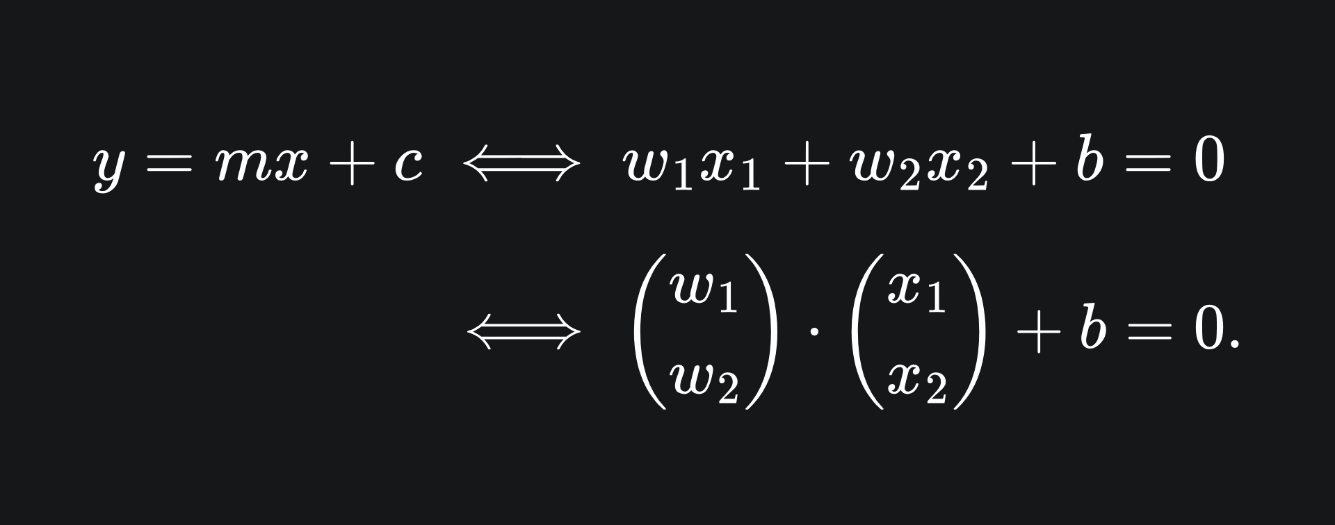
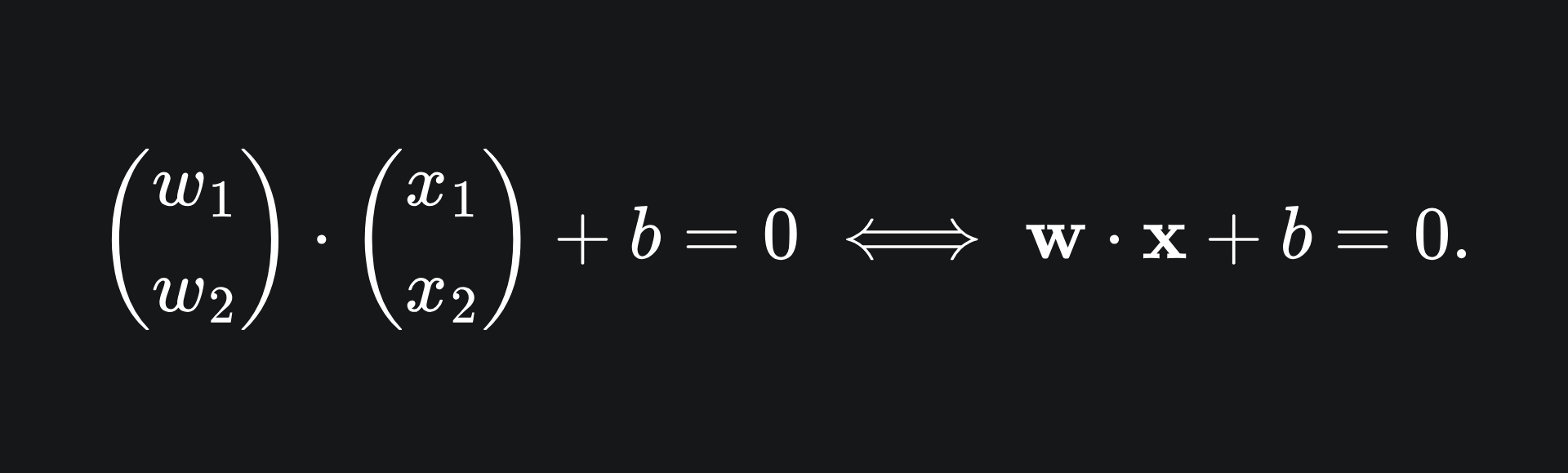
The notation on the right hand side allows us to write the equation using vectors. As we did in our discussion of multiple linear regression, we can use bold letters to represent vectors:

\(\begin{pmatrix} w_1 \\ w_2 \end{pmatrix} \cdot \begin{pmatrix} x_1 \\ x_2 \end{pmatrix} + b = 0 \iff \textbf w \cdot \textbf x + b = 0.\)

As it so happens, the vector w is perpendicular to the line. We won’t prove this, but will instead verify it for the simple example of y=x. We can convert y=x into the form wx+b=0 form as follows:

\(\begin{align} y=x & \iff x-y=0 \\ & \iff 1\cdot x_1 + (-1) \cdot x_2 + 0= 0 \\ & \iff \begin{pmatrix} 1 \\ -1 \end{pmatrix} \cdot \begin{pmatrix} x_1 \\ x_2 \end{pmatrix} + 0=0. \end{align}\)

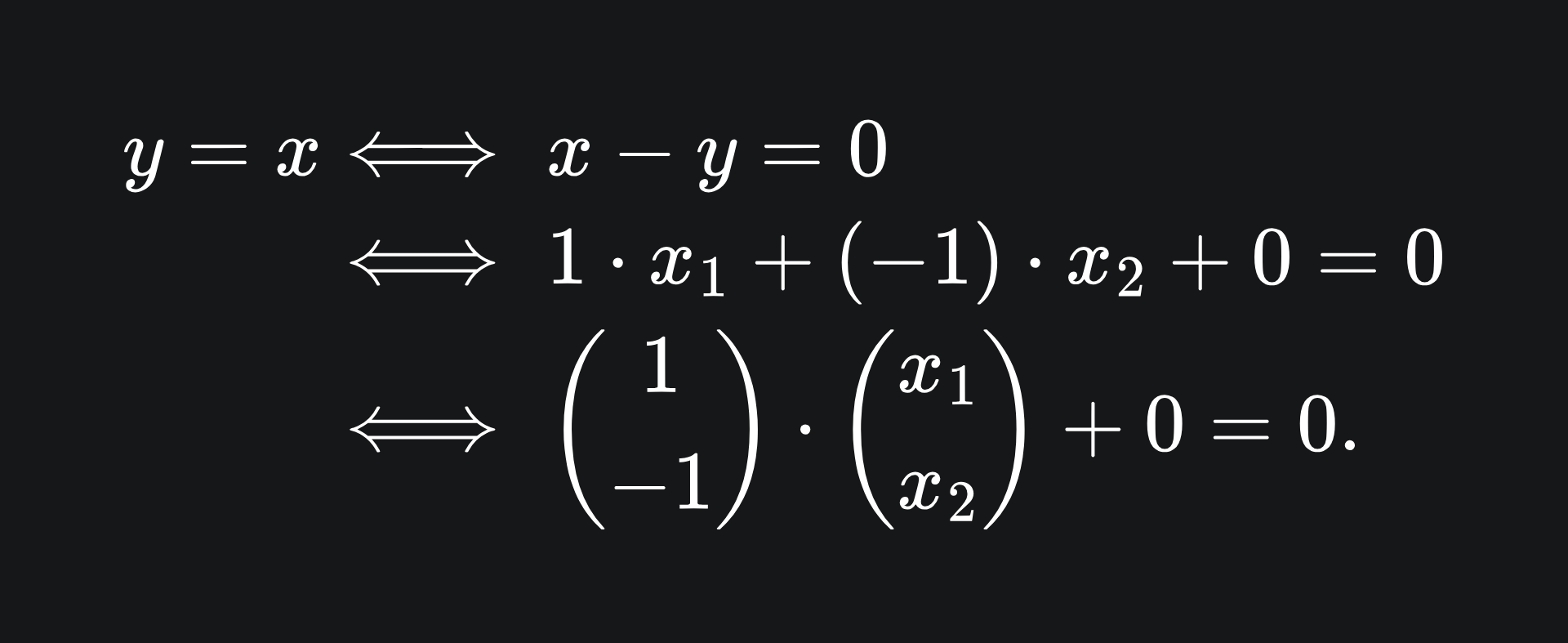
This vector equation tells us that any coordinate (x_1, x_2) which satisfies the above equation will lie on the line y=x. The line y=x is plotted below, along with the vector w, which is indeed perpendicular to the line:

When using the wx+b=0 form for the equation of a hyperplane, the vector w is always perpendicular to the line.

This formulation is useful, because for any point above the line, we have that

\(\textbf w \cdot \textbf x + b > 0,\)

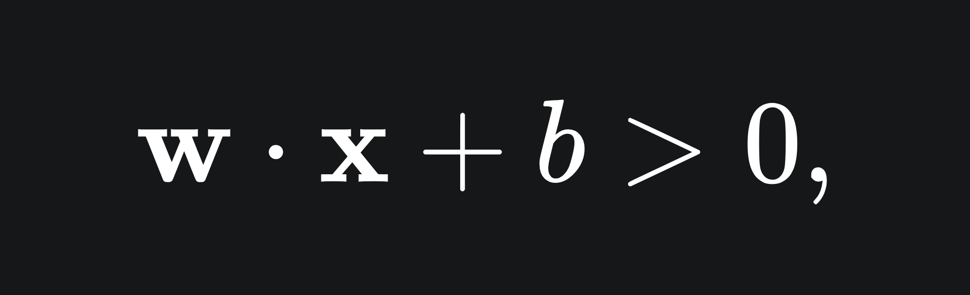
and for any point below the line, we have that

\(\textbf w \cdot \textbf x + b < 0.\)

If this is not clear, plug in some values for x_1 and x_2 in the above example.

Note that (you might have seen this coming) this setup extends to n dimensions. Namely, an (n-1)-dimensional hyperplane in n dimensional space can be written as

\(\textbf w \cdot \textbf x + b = 0,\)

where

\(\textbf{w} = \begin{pmatrix}w_1 \\ \vdots \\ w_n \end{pmatrix} \text{ and } \textbf{x} = \begin{pmatrix}x_1 \\ \vdots \\ x_n \end{pmatrix}.\)

Support vectors

We need to define some extra terminology relevant to the SVM.

Let’s represent our dataset as

\(\{ \{ \textbf{x}_1, y_1 \}, \{ \textbf{x}_2, y_2 \}, \dotsc, \{ \textbf{x}_n, y_n \} \},\)

where each x_i is a row of data with corresponding label y_i. Suppose each y_i takes a value in the binary set {+1,-1}. To construct a separating hyperplane for this data of the form wx+b=0, we require

\(\begin{align} \textbf w \cdot \textbf x_+ & + b > 0, \\ \textbf w \cdot \textbf x_- & + b < 0. \end{align}\)

for any data point x+ with label +1, and any data point x- label -1. That is to say, we want all data points of label +1 to be above the hyperplane, and all data points of label -1to be below.

We define the support vectors to be the pair of vectors that are closest to either side of the hyperplane. One will be a +1 vector and the other will be a -1 vector.

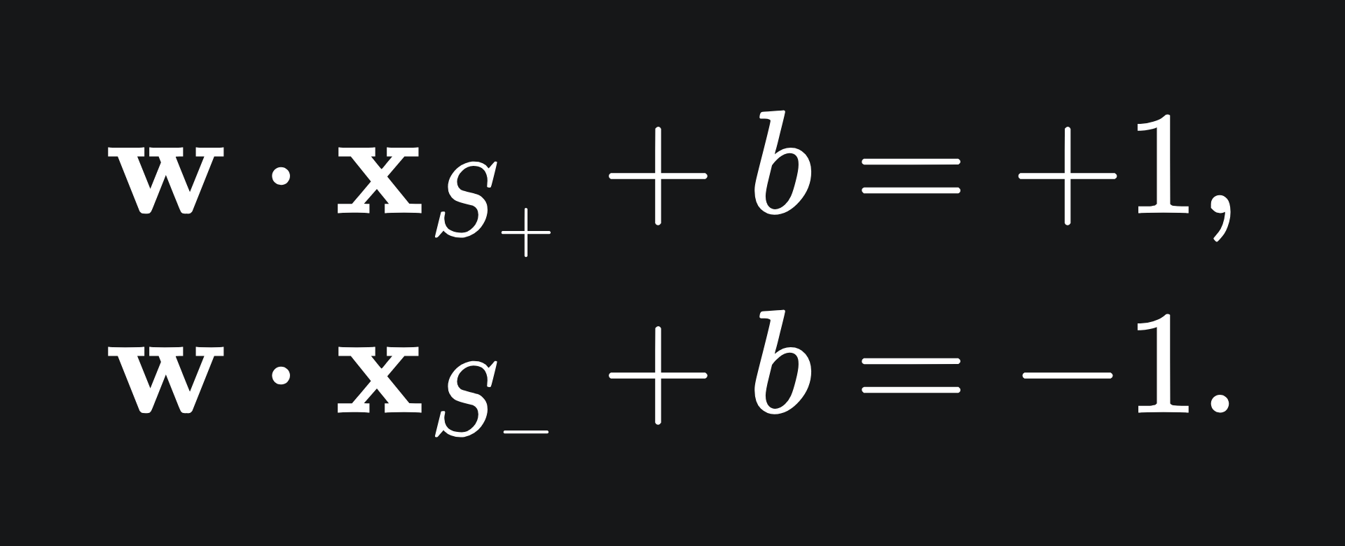
Let’s call the support vectors S+ and S- respectively. Since these support vectors will lie above and below our separating hyperplane, we already know that

\(\begin{align} \textbf w \cdot \textbf x_{S_+} & + b > 0, \\ \textbf w \cdot \textbf x_{S_-} & + b < 0. \end{align}\)

In the end, we will want these supports specifically to satisfy

\(\begin{align} \textbf w \cdot \textbf x_{S_+} + b = +1, \\ \textbf w \cdot \textbf x_{S_-} + b = -1. \end{align}\)

Therefore, we are looking for w and b that satisfy the below, for general x+ and x-:

\(\begin{align} \textbf w \cdot \textbf x_+ + b \geq & +1, \\ \textbf w \cdot \textbf x_- + b \leq & -1. \end{align}\)

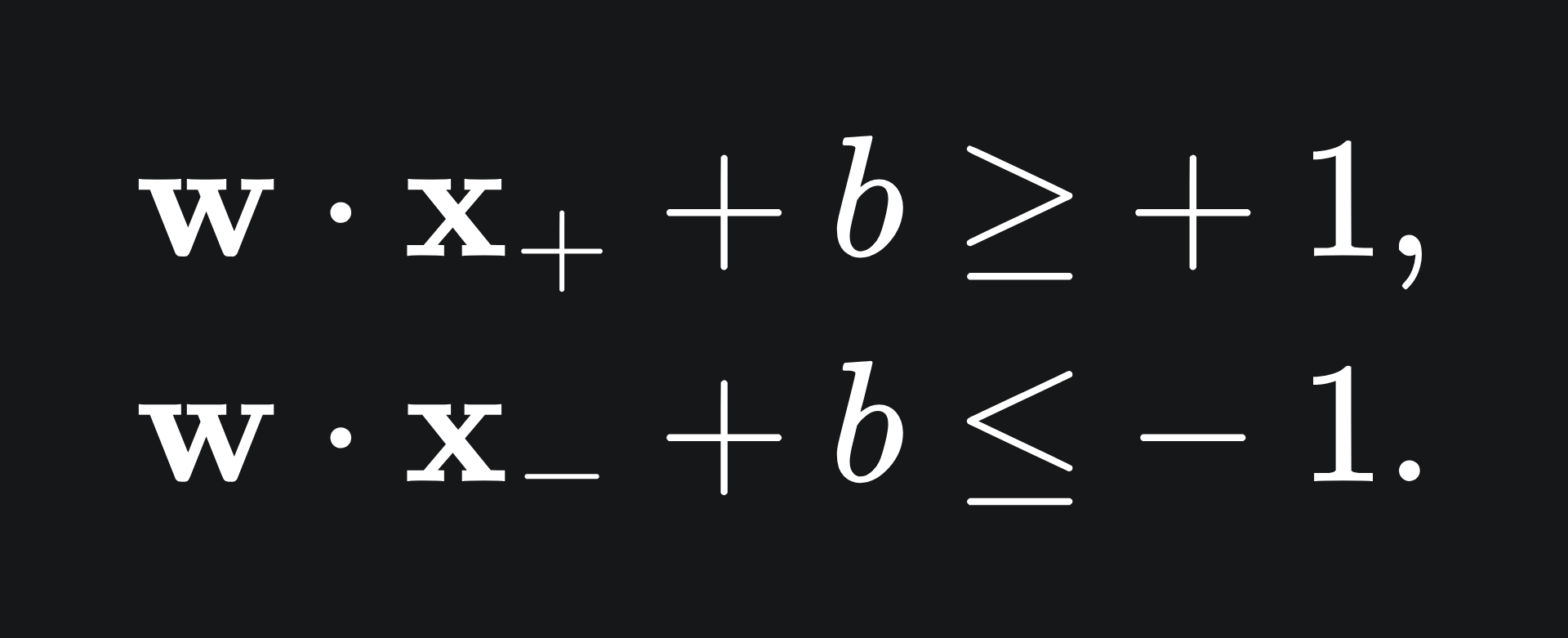
(The above become equalities for the supports S+ and S-.)

We can write these inequalities compactly in just one inequality:

\(\begin{align} y_i \cdot (\textbf w \cdot \textbf x_i + b) \geq 1. \end{align}\)

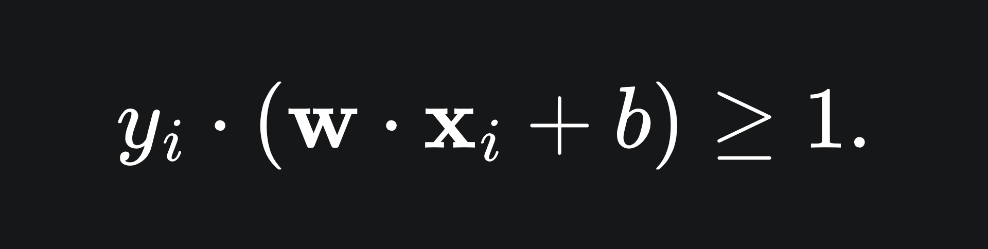
This clearly works for the ‘+1’ points because in these cases y_i=1. But for the points below the line, we have y_i=-1, and the product of two negative numbers is positive.

The margin

The margin of the SVM is the distance between the separating hyperplane and the two support vectors. The perpendicular distance between a support vector and the separating hyperplane is given by

\(\frac{1}{\| \textbf w\|} = \frac{1}{\sqrt{w_1^2+\dotsc+w_n^2}}.\)

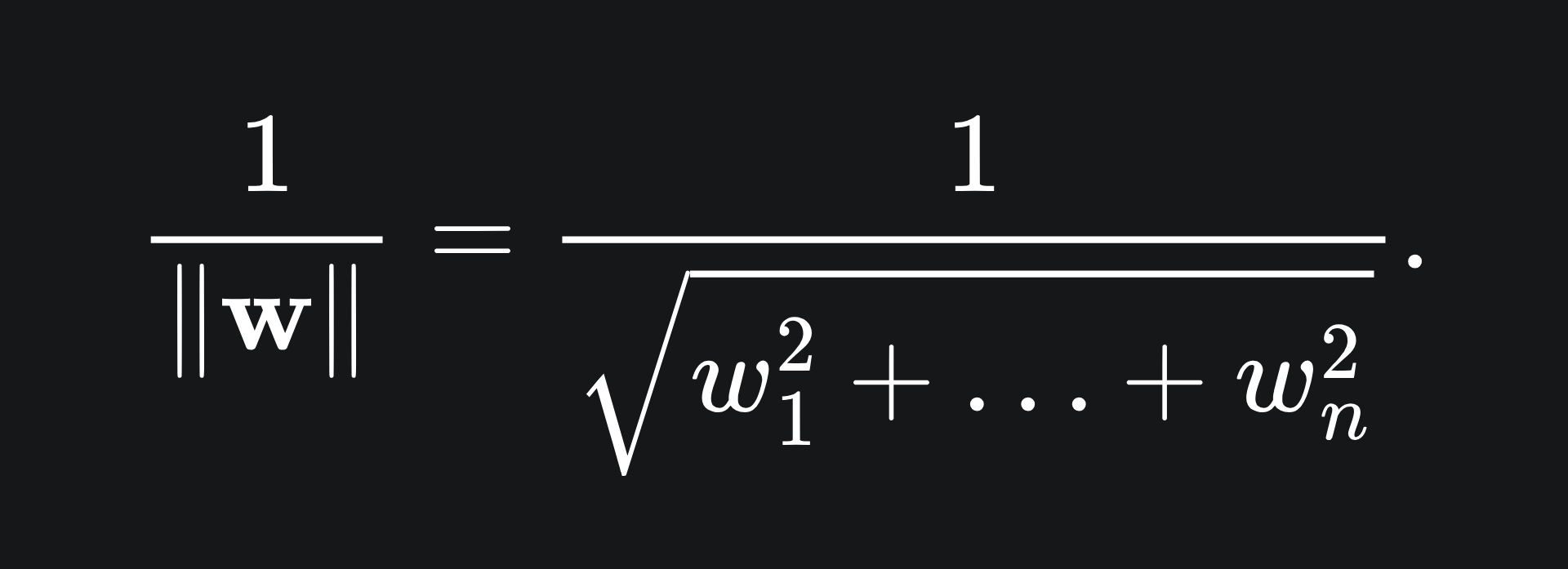
We will derive this formula in a future article. ³

As there are two support vectors, the margin is just double the above quantity.

In the meantime, have a think about the following: would it be better for an SVM to have a large margin or a small margin?

Well, the larger the margin, the more easily the SVM can classify unseen points, because the distinction between the two classes of data will be clearer. So we in fact wish to maximise the margin of the SVM.

Visual demo

Here is a video example to help illustrate everything we have covered so far. In particular, we have a dataset for which the hyperplane y=-x is used to separate the data into the two classes. Moreover, the support vectors S+ and S- have coordinates (4,-2) and (-3,1) respectively.

Finding an ‘optimal’ hyperplane

What makes a chosen hyperplane ‘optimal’?

Given the previous sections, it’s clear that we want a hyperplane which:

1. Correctly separates the data into the two categories.

2. Provides the largest margin possible.

The first condition gives us a constraint, and the second condition provides us with an objective to optimise. Combining this leaves us with a so-called constrained optimisation problem:

\(\begin{align} \text{Maximise} & & \frac{2}{||\textbf w||} \\ \text{Subject to} & & y_i(\textbf w \cdot \textbf x_i + b) & \geq 1. \end{align}\)

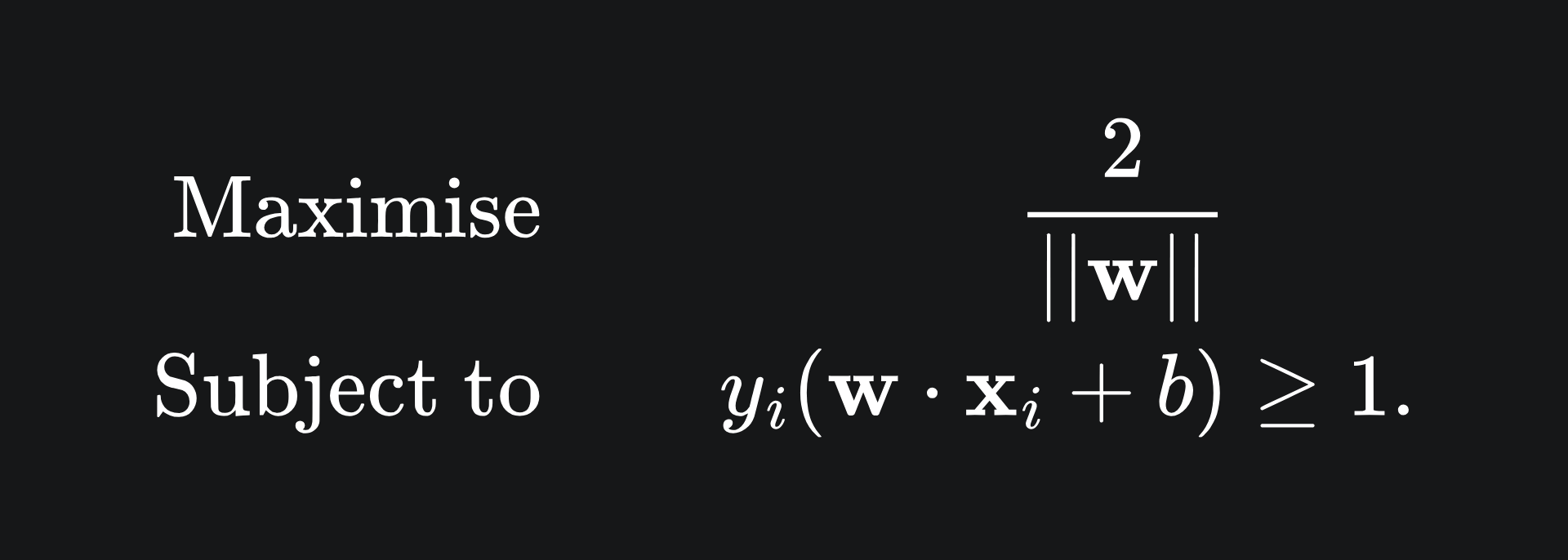
Solving this problem requires some tools that are beyond the scope of this article. ⁴

What if the data isn’t linearly separable?

In reality, it will not always be possible to partition your data in n-space. It turns out that there are some solutions for this with the SVM…

… but we’ll discuss this next week, so stay tuned!

Packing it all up

If you made it this far, then well done! The good thing about the SVM is that it relies on geometry, so we can look at pretty pictures to better understand it. The bad thing about the SVM is that it relies on geometry, so if you don’t like working with vectors, it can feel somewhat difficult to approach compared to some of the other algorithms we’ve covered.

Anyhow, here’s a summary of what we’ve learned:

• The Support Vector Machine is a supervised learning algorithm which aims to find the most ‘optimal’ separating hyperplane for a dataset of two labels.

• The support vectors are the pair of vectors that are closest to either side of the separating hyperplane.

• The margin is the distance between the separating hyperplane and the two supports. We want to maximise the margin of the separating hyperplane for the sake of classifying new points.

Training complete!

I really hope you enjoyed reading!

Do leave a comment if you’re unsure about anything, if you think I’ve made a mistake somewhere, or if you have a suggestion for what we should learn about next 😎

Until next Sunday,

Ameer

PS… like what you read? If so, feel free to subscribe so that you’re notified about future newsletter releases:

1. The logistic regression model is used for regression rather than classification in the context of statistics- the stuff that I say in these articles usually pertains to the context of ML, not necessarily other disciplines.

2. Recall that ‘supervised’ means we have a labelled dataset, where the goal of the model is to predict the labels given the data features.

3. This is shorthand for “This article became too long and I’ll need a part 2 to do justice to the SVM”. But I’m sure part 2 will be a banger 😎

4. Keen readers should look into Lagrangian optimisation. Otherwise, numerical methods can be leveraged to converge upon an optimal solution.