
Adaptive learning rates for gradient descent
Explaining the maths behind the Adagrad, RMSProp and Adam optimisers.

Hello fellow machine learners,
Last week, we learned about both Stochastic Gradient Descent (SGD) and mini-batch gradient descent, and how they can resolve the issues of regular gradient descent, particularly within the context of training neural networks. Quick recap on the pros and cons of these techniques over regular gradient descent:
✔️ Uses less system memory, since we don’t need to load the full dataset for each gradient descent step.
✔️ Can run more quickly, because we’re leveraging data samples rather than the full original dataset.
❌ Due to the fact that samples of data cannot necessarily capture the main patterns within the full dataset on their own, parameter updates from the SGD and mini-batch methods can be more noisy.
❌ As a consequence of the above point, batching procedures are more sensitive to the learning rate.
Today’s article will focus on the learning rate of the gradient descent algorithm. Regardless of whatever gradient descent algorithm you use, the learning rate is important, because it controls the magnitude of the descent steps taken at each iteration of the corresponding algorithm.
Our discussion will revolve around one solution for optimising the learning rate when trying to reduce the loss of an ML model with respect to the model’s parameters.
Let’s get to unpacking!
Fixed learning rates
The simplest learning rate implementation is that of a constant value, usually a decimal between 0 and 1. The use of a fixed learning rate means that the size of each descent step is the same. Although easy to understand and use, the gradient descent algorithm’s current/previous step progress is not taken into account. We’ll see why that might be useful in the following subsections.
For now, consider the following simple, albeit somewhat contrived, loss function:
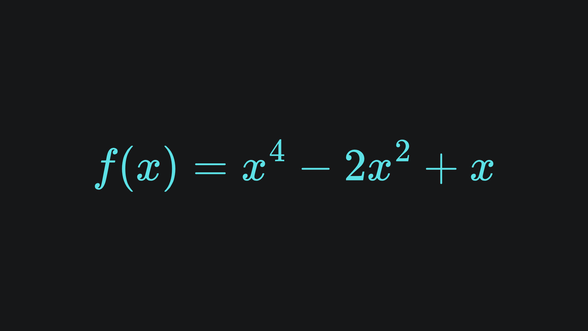
Here is what the main part of it looks like:
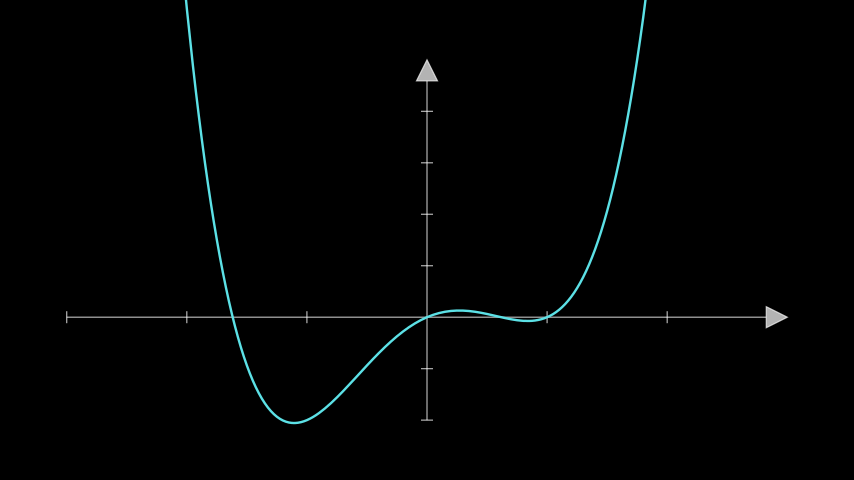
We can imagine that x is the single model parameter that the loss function is written with respect to.
If we wanted to minimise the value of this function with respect to the parameter x, we could apply gradient descent. However, there are two minimum points in this function. It’s clear visually that the leftmost minimum point is the global minimum point, but note that we’re not usually able to just plot loss functions and spot minima like this so easily in practice. Nevertheless, it’s good to see the point that we want to end up close to.
The following simulation depicts 8 steps of gradient descent for a pair of points with different initial positions, with the yellow point using a fixed learning rate of α=0.5, and the orange point using a fixed α=0.8. Let’s see what happens:
Hmm… interesting. Let’s remark on some of what just happened:
💡 Although the yellow point converges upon a minimum point, it isn’t the global minimum point. The main reason for this is the fact that we initialised the yellow point rather poorly. If it started a bit more to the left, then gradient descent probably would’ve steered us in the correct direction. But again- you are often not able to visualise loss functions in this manner, if at all, in reality.
💡 The orange point begins by moving in the correct direction, towards the global minimum point. The first gradient step looks great! The next step goes… well, uh, I’m not too sure. From there onwards, it’s hard to keep track of the orange point. In fact, it escapes my plot entirely! This happens because the step size is far too large, and the algorithm struggles very early on with course-correction as a result.
In terms of the first insight, we could run gradient descent for a bunch of points with different initialisation positions, then take the average of the final coordinates in the hope that we’re not always ending up at the non-global minimum. But even if we implement this, the second insight shows us that, unless we know exactly what the loss function looks like (as we do here), there’s quite a lot of guesswork involved. And if we’re struggling with a contrived quartic loss function, then we have no hope for minimising loss functions in real-world neural networks, which have far more complex surfaces and many more parameters involved.
Let’s try using α=0.1 for both instead and see if the performance improves:
This time, the orange point converges well to the global minimum value. And given the initialisation, the yellow point still moves toward the local minimum as before. However, this time, the descent steps are too small, and so the yellow point doesn’t reach its destination in the 8 steps.
From all this, we can conclude that a fixed learning rate simply isn’t robust enough in practice. Something more powerful is needed!
Adaptive learning rates
Hopefully you’re convinced thus far that a static learning rate is insufficient for our machine learning requirements. If so, read on to learn about learning rates that can take different values for each gradient step.
Suppose that your ML model has parameters w1, w2,…, wn. The adaptive learning rates from here onwards will rely on the values of previous gradient values. Thus, we’ll endow each model parameter with a history indexed by time t. That is to say, wi,t represents the value of model parameter i at time t. Each adaptive learning rate will be defined in a general way like this.
For us, gradient descent for the model parameter wi at time t is given by
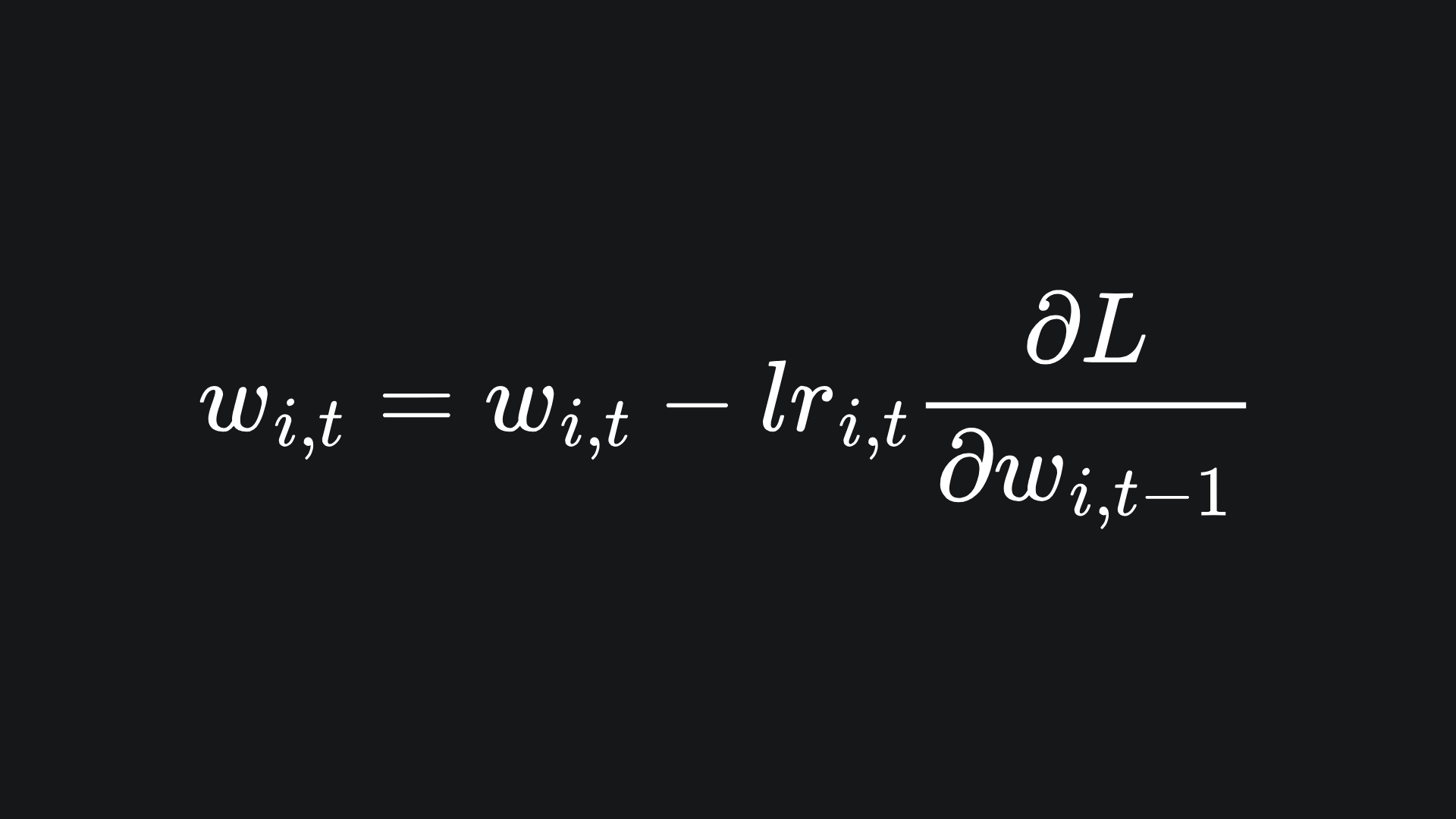
where the learning rate lri,t will depend on the adaptive learning rate method. We’ll discuss some examples below!
(NB since my code example used a one-dimensional function, i.e. only one model parameter, you can ignore the i if that helps to simplify things if you want.)
Adagrad optimiser
The adaptive gradient algorithm (abbreviated to Adagrad) aims to adjust the learning rate for each distinct model parameter, according to the parameters’ previous values.
Adagrad uses a separate learning rate for each model parameter. The learning rate of Adagrad is defined as:
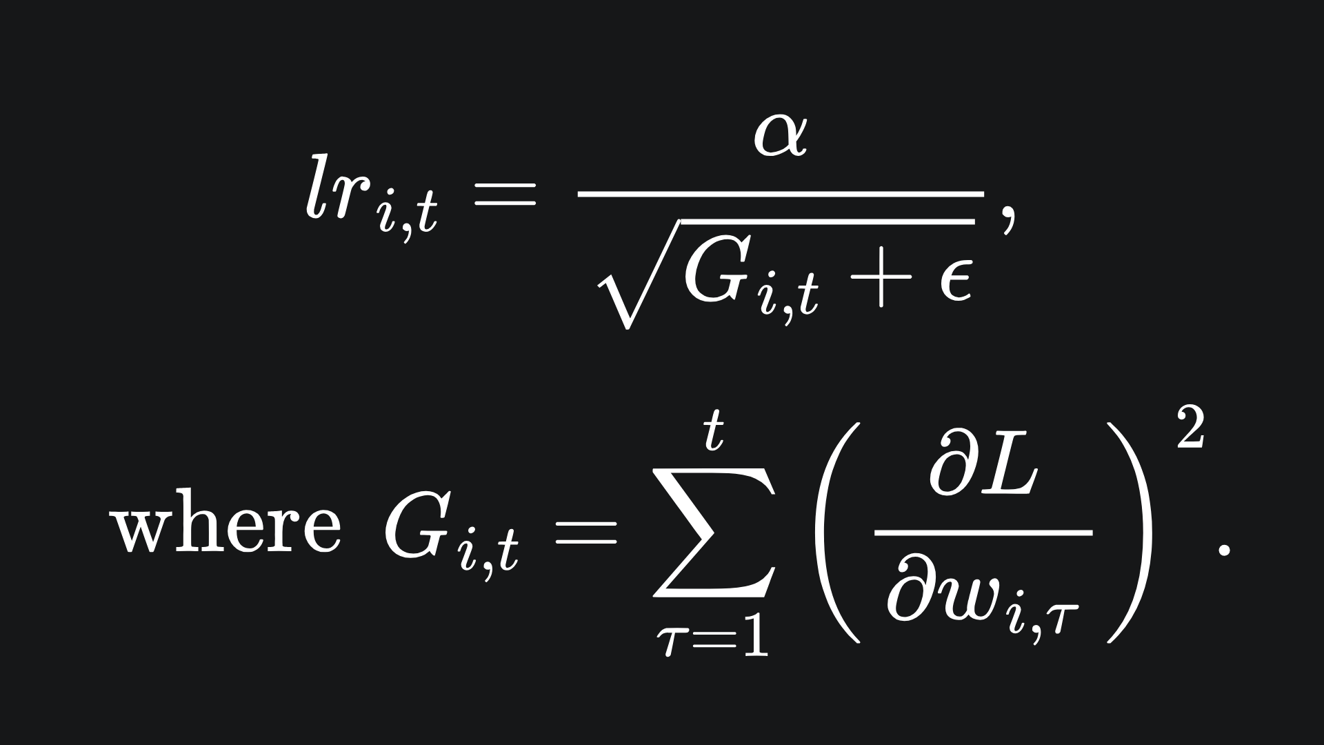
So Gi,t is the sum of squared gradients of parameter wi up to time t. So for each gradient descent iteration, evaluate the new learning rate and use this to compute the next parameter value. The parameter ϵ is a small value that helps avoid division by zero.
As the sum of squared gradients increases, the learning rate decreases. The sum of squared gradients will naturally increase with more algorithm iterations. Thus, Adagrad forces smaller and smaller gradient steps as the algorithm propagates.
Also, notice that α is a hyperparameter for Adagrad. So you can play around with it and see what happens to the algorithm’s performance.
In the following animation, we test the performance of Adagrad against the fixed learning rate of α=0.1 for the starting point x=0.1:
Hmm… the fixed learning rate is actually doing a better job here! The issue arises from the fact that Adagrad penalises future step sizes too harshly.
RMSProp optimiser
The Root mean Square Propagation (RMSProp) optimiser aims to fix Adagrad’s issue of overly penalising gradient step sizes. Here is what the RMSProp learning rate looks like:
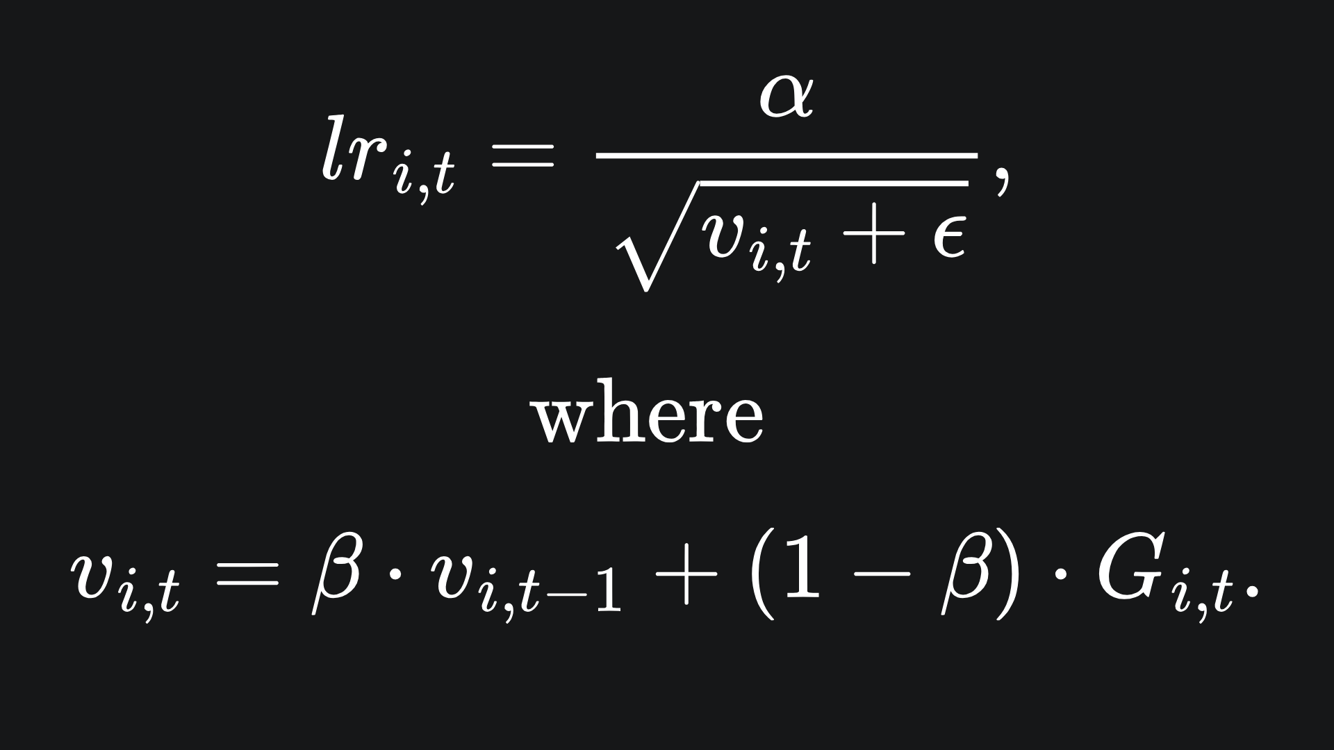
While Adagrad provides equal importance to each gradient in the sequence, RMSProp gives more weighting to more recent gradient values. This weighting is controlled by the parameter β, whose value is taken between 0 and 1. The closer β is to 1, the more weighting is given for the recent gradients. In practice, it is recommended to keep β close to 1 for this reason.
The formula for vi,t is what’s known as an exponential moving average1 of the squared gradients. And don’t forget that, like with Adagrad, Gi,t is the sum of squared gradients of parameter wi up to time t.
Let’s compare the performance of Adagrad and RMSProp with α=0.1 and β=0.9, starting at x=0.1:
This is much better- RMSProp is able to take larger steps at the start, and then slows right down as we get to the desired global minimum point.
Adam Optimiser
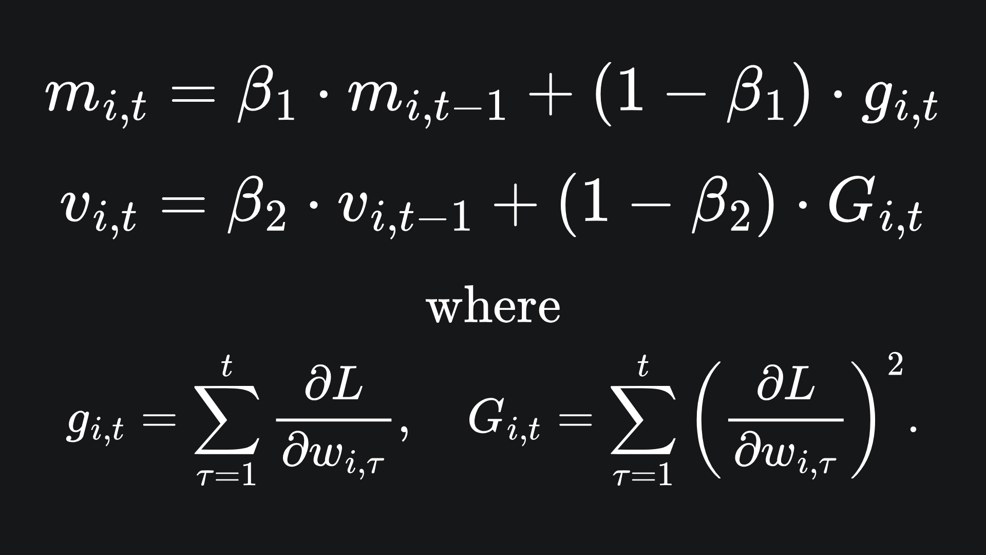
The Adaptive Moment Estimation (aka Adam) optimiser builds upon RMSProp by incorporating something called momentum. Adam keeps track of not only the exponential moving average of squared gradients (just like RMSProp), but also the exponential moving average of regular gradients. Adam uses a separate beta parameter for tracking each of these moving averages independently:
On top of this, we implement bias correction terms:
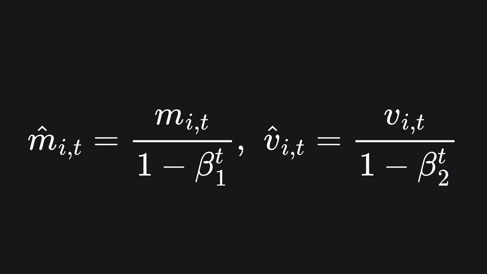
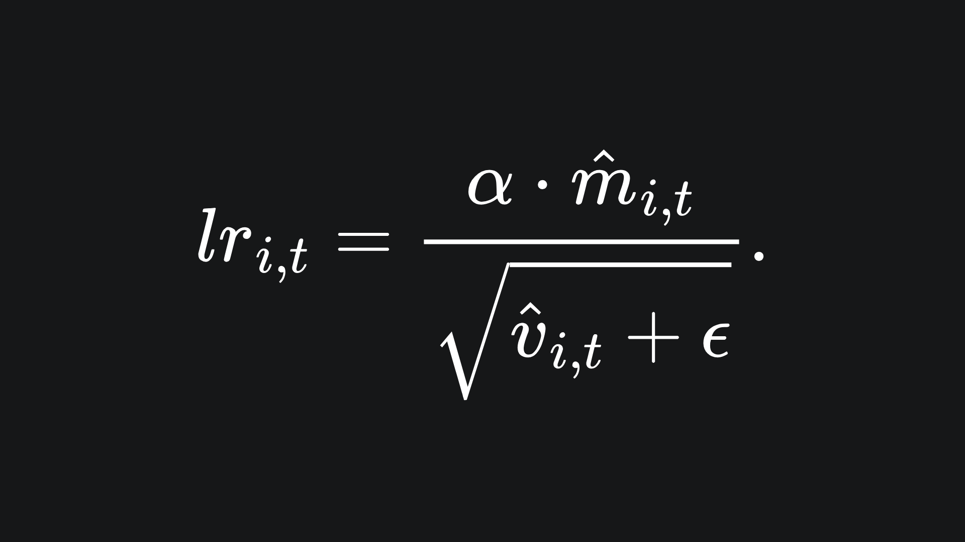
The utility of these is explained in the next subsection. For now though, these values are incorporated into the learning rate as follows:
Let’s take a look at RMSProp vs Adam with α=0.1, β=0.9, β1=0.9 and β2=0.999, with a starting position of x=0.1. Note that I have chosen β1=0.9 and β2=0.999 since these are the default parameters as per the PyTorch implementation.
Both optimisers find the minimum point, but RMSProp actually converges to the global minimum faster. Let’s test out the optimisers on a more complicated function. What about2:
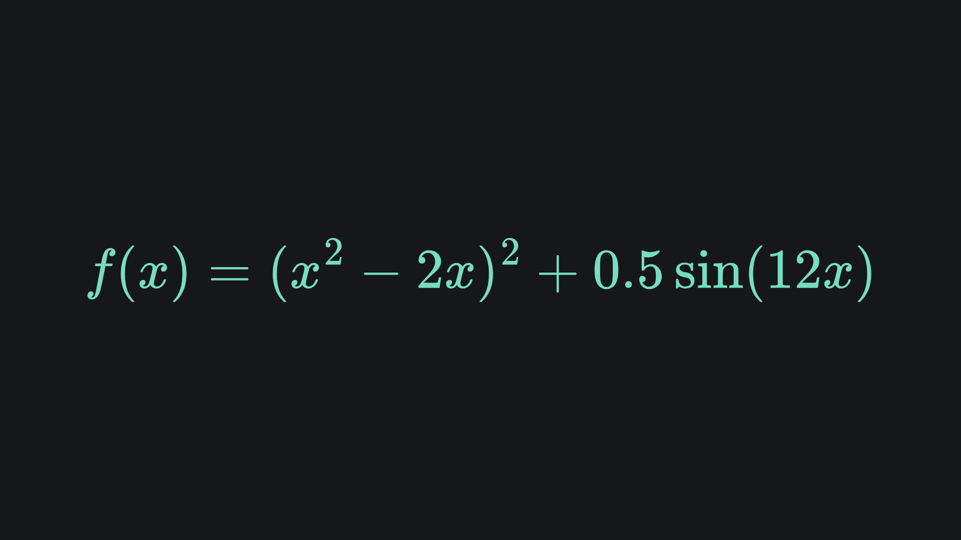
Let’s see how the optimisers perform, this time with α=0.05, x=0.5 and all other parameters the same as before:
We observe that the momentum component of Adam pushes it beyond the (non-global) local minimum point that RMSProp falls susceptible to.
Why bias correction for Adam?
For the initial iterations of the exponential moving average technique, updates are more biased towards taking unnecessarily small values. The method used above helps to solve this problem and, as the value of t increases, the effect of bias correction fizzles out and so doesn’t interfere with future predictions.
Check out the following short video from Andrew Ng which helps explain this concept within the context of time series forecasting:
Packing it all up
I encourage you to play around with the code, which you can find at my GitHub here. Experiment with the learning rates, initialisation positions and number of steps, and see what happens to the convergence of the various learning rates!
And now for the regular roundup:
📦 Adagrad adjusts learning rates by summing up the squared values of previous gradients. This means that every extra Adagrad step reduces in magnitude. This is helpful if you want the gradient descent to take smaller steps every time, but size reduction may occur prematurely.
📦 RMSProp resolves Adagrad’s issue of overly reducing step sizes by applying an exponential moving average technique. This places greater importance on the most recent gradient updates, making for a more robust adaptive learning rate.
📦 The Adam optimiser extends RMSProp by incorporating momentum. Along with bias correction, this can help Adam to look beyond the local optima that can trip up RMSProp.
Training complete!
I hope you enjoyed reading as much as I enjoyed writing 😁
Do leave a comment if you’re unsure about anything, if you think I’ve made a mistake somewhere, or if you have a suggestion for what we should learn about next 😎
Until next Sunday,
Ameer
PS… like what you read? If so, feel free to subscribe so that you’re notified about future newsletter releases:
Sources
My GitHub repo where you can find the code for the entire newsletter series: https://github.com/AmeerAliSaleem/machine-learning-algorithms-unpacked
“Adam: A Method For Stochastic Optimization”, by Diederik P. Kingma and Jimmy Lei Ba: https://arxiv.org/pdf/1412.6980
Unrelated side note: exponential moving averages also see the light of day within the context of time series forecasting.
Full disclosure: I had some help from ChatGPT to help me come up with a suitable function.
Great illustration of the RMS prop optimization.