LLM evaluation with confidence intervals: a statisical view

The Central Limit Theorem and its application to confidence intervals for the "true" mean LLM eval score.

Hello fellow machine learners,

Last week, we extended the concept of LLM-as-a-judge via Chain of Thought prompting and the G-EVAL framework. You won’t need that article’s contents for today’s necessarily, but here’s the link if you’re interested:

Chain of Thought prompting and G-EVAL: improvements to LLM-as-a-judge

In this article, we’re going completely left-field to consider LLM evaluation from a statistical perspective. Over the past few weeks, we’ve looked at performance metrics for LLM evaluation across a few research papers, which reported metrics in tabular formats. And while experiments may have been repeated to check for fluked results, they all lack one thing: confidence intervals.

Loosely speaking, a confidence interval indicates a region within which a variable’s “true value” is likely to reside, although the true definition is a little more nuanced than that. Nevertheless, this offers a more robust and scientific approach to LLM evaluation, because it allows us to capture the underlying uncertainty in our results. More on this in the next section.

Confidence intervals arise from statistical theory and, for the record, I hated statistics at college¹. I didn’t understand the methods we used for the likes of hypothesis tests, and the pedantic language used to define things like confidence intervals felt super complicated. But now that I’ve undergone the baptism of fire that was my undergraduate mathematical education, I think that now is as good a time as any to revisit these topics and find out whether the concepts are any more appealing to me, or at least make a bit more sense intuitively.

Or, you know, maybe I’ll just be a statistics hater for life.

Excited? Then let’s get to unpacking!

Motivation

Let’s set up a figurative scenario to aid with motivation. Suppose that you’re at an arcade playing a game involving a lever. You are told that the lever gives you some money every time it’s pulled, but not necessarily the same amount every time, as the monetary reward follows an unknown probability distribution with mean μ and variance σ. The arcade game’s premise is that of a question: how would you go about evaluating/estimating the mean μ?

I’m well aware that this scenario is entirely unrealistic- no arcade will be giving out cash prizes for free. So, let’s replace the lever with an LLM prompt, and the money with the evaluation score for the LLM’s output. All of a sudden, the problem transforms into the very question we’ve been investigating over the past few weeks!

Let’s be a bit more specific: we know that LLM outputs are inherently stochastic, which means that the output quality is subject to change, even if we’re passing in the same prompt each time. To that end, we want to know the true value of the mean LLM eval score, which can be denoted as μ. An example use case could be where we aim to evaluate how well the LLM summarises text. In this case, μ could represent the LLM’s evaluation score (out of 5) across all possible candidate summary texts. This is the best we can get to a ground-truth value for the LLM’s efficacy in summarising text data.

As in the arcade example, here’s the same question again: how do we estimate the value of the true mean μ? To be super accurate, we’d have to pull the lever an infinite number of times and take the average, but this is far from practical. As a compromise, we could pull the lever a few times, i.e. provide a few different prompts to the LLM, and take the average. This is what we called the empirical (or sample) mean, and would likely provide a reasonable estimate for the true mean μ. But how reasonable would this estimate for the true mean be? Due to LLM stochasticity, there will be variance in the scores from the sample that we’d need to take into account.

First things first: the average of a set of eval scores for the LLM, the sample mean, can be denoted s̄. We can represent each individual LLM output score as s_i, corresponding to input questions q_i:

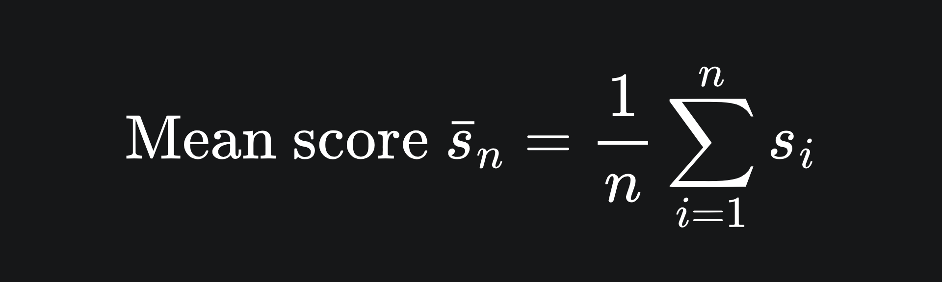
Now our main question is: how good an estimate is s̄ of the true LLM mean score μ? This sounds difficult to figure out, because we don’t know anything about the underlying probability distribution of the LLM’s outputs.

What we need is a technique that generalises to any LLM or, to be more precise, to any unknown probability distribution. Introducing the…

Central Limit Theorem (CLT)

Suppose that X₁, X₂,…, X_n are independent and identically distributed random variables, each with finite mean and non-zero finite variance. Then the random variable defined as

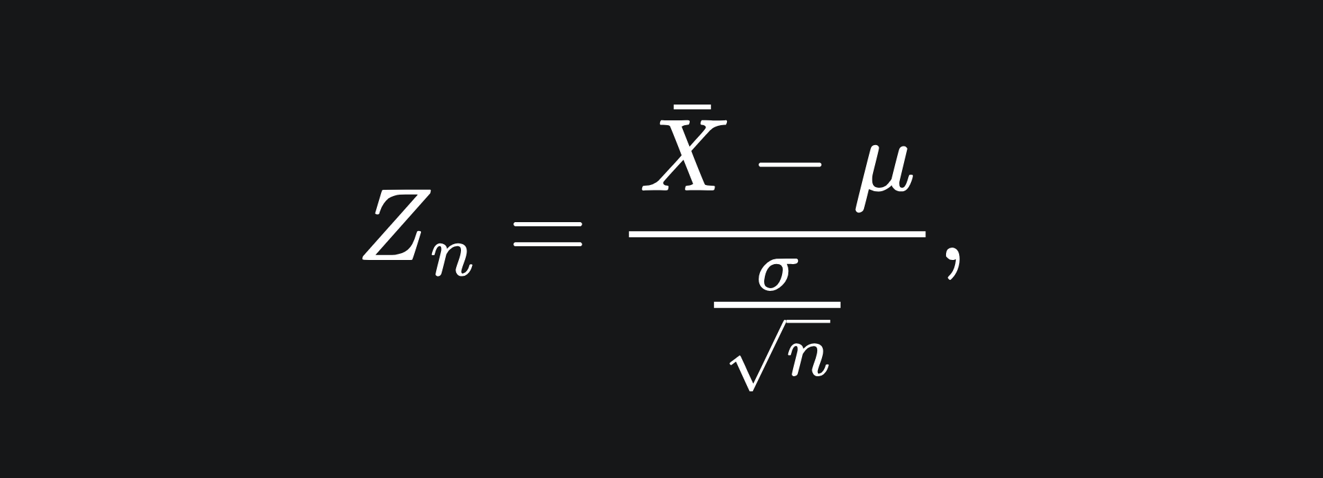
which I will call the Z-score of the sample mean, converges in distribution to the standard Gaussian. This is represented algebraically as

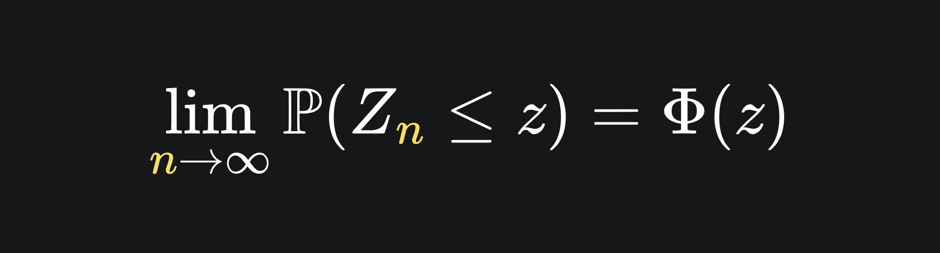
where Φ is the cumulative density function of the standard Gaussian.

This result is known as the Central Limit Theorem (CLT), one of the most important results in all of statistics. It’s a statistics Hall of Famer, if you will.

The above description states the CLT in its most general form. There’s another (less rigorous) version that may be easier to interpret: assuming that the conditions specified at the top of this section are satisfied, the sample mean is approximately Gaussian, with the following parameters:

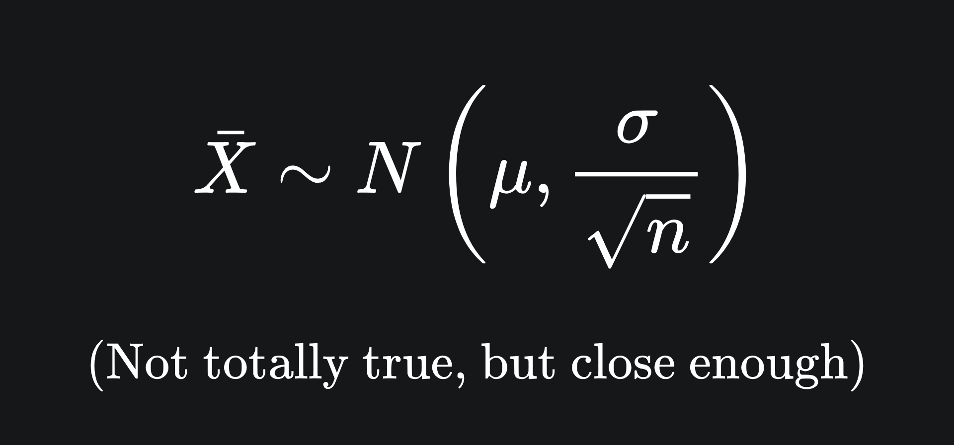
However, we’ll stick with the original version, because it’s useful to compare things to the standard Gaussian distribution, as we’ll see in the next section.

Visualisation of the CLT

Let’s play around with some visualisations to better understand what the CLT is telling us.

Recall the exponential distribution, defined as:

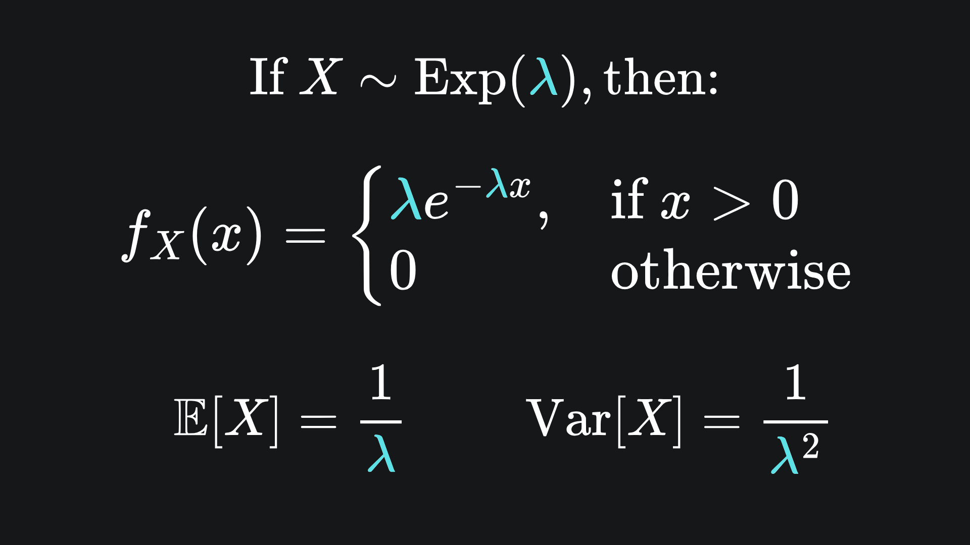
We will investigate the mean of a sample of n iid exponential random variables of parameter λ=2. The idea is to consider 5000 realisations of this sample mean, compute the corresponding Z-score and plot the probability density. (The choice of 5000 is arbitrary, but the more the better!). By the Central Limit Theorem, we expect that our sample mean Z-score will resemble the standard Gaussian for large values of n. This is described rigorously with the following:

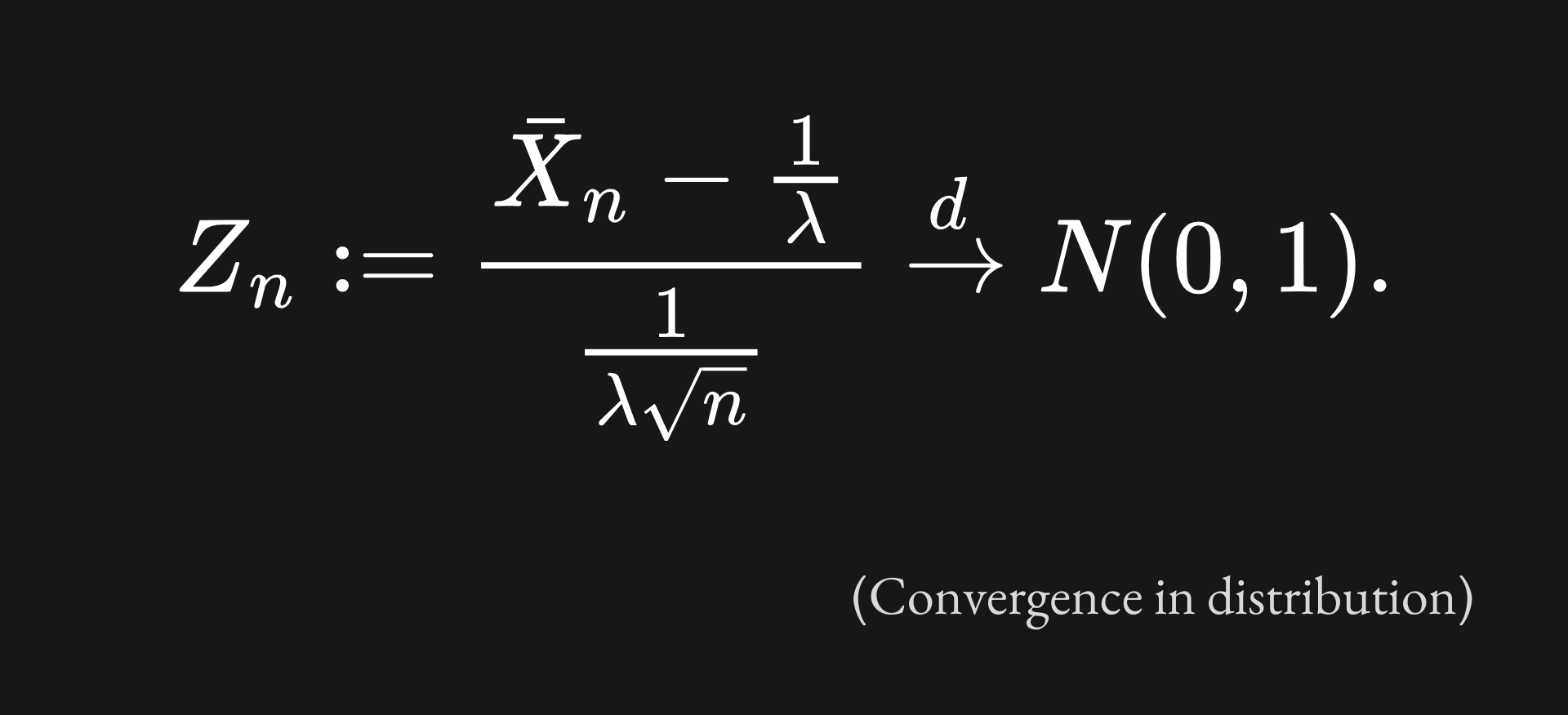
Now to investigate this empirically. In the following visual, this is first done for a single sample (n=1), which we then increase to n=10, n=20, n=30 and finally n=1000. The original exponential distribution is plotted (blue), as is the standard Gaussian distribution (red) for comparison.

This verifies precisely what the Central Limit Theorem predicted! Remember that this holds because our collection of exponential random variables are independent and identically distributed, plus the distribution has finite mean and variance.

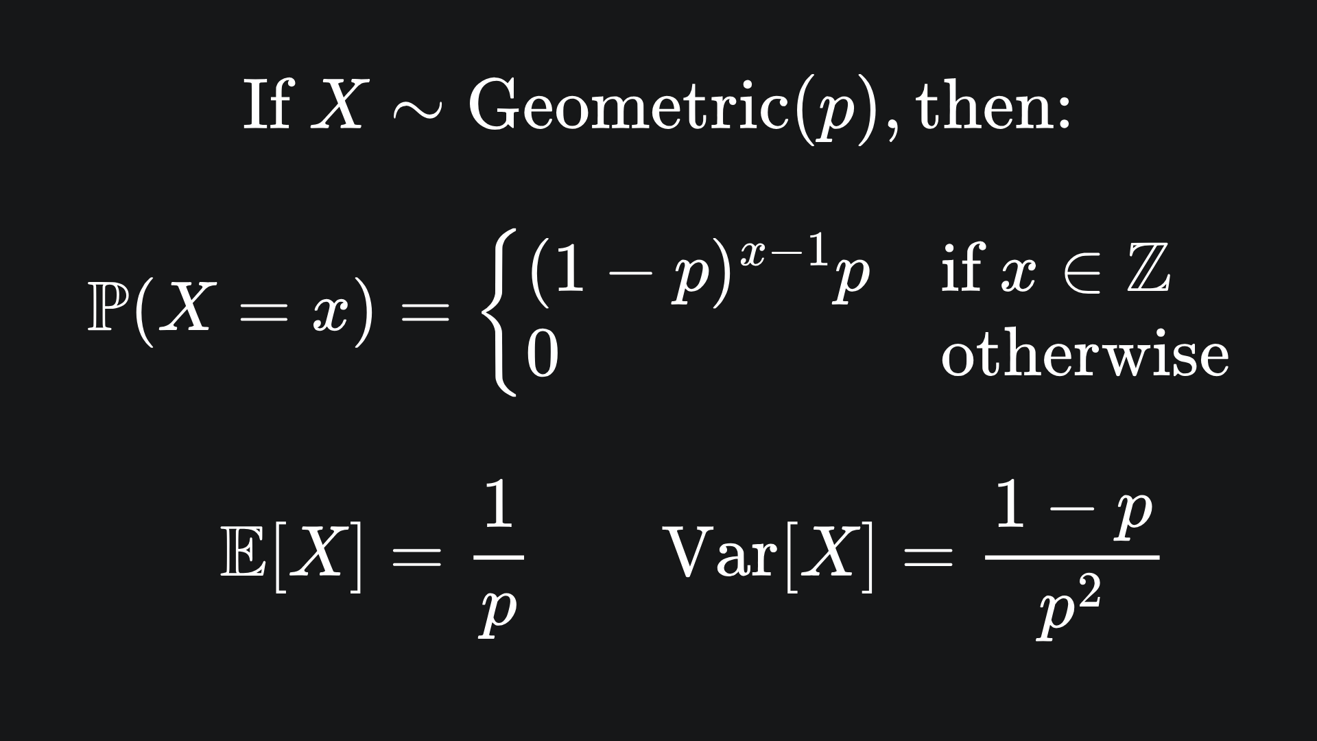
What’s fascinating is that the CLT holds not just for continuous random variables, but discrete ones too! Let’s look to the geometric distribution as an example:

As before, we expect that the sample mean Z-score, defined here as

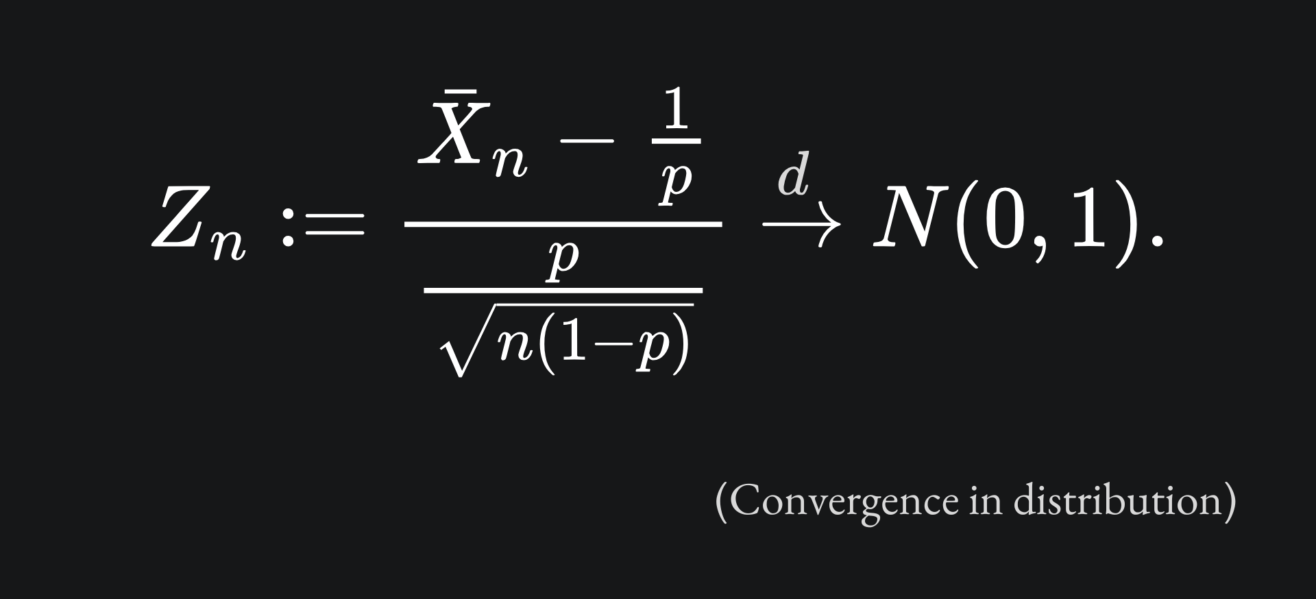
will converge in distribution to the standard Gaussian. Let’s repeat the empirical investigation from before and see what happens. Note that I’ve plotted the probability mass function as a line graph here, but a histogram would have been more appropriate since the geometric distribution is discrete:

If you think about it, this is an insanely powerful result; assuming that certain conditions are satisfied, the sample mean begins to approximate a Gaussian, regardless of the original probability distribution. For example, even though the exponential distribution is skewed, the sample means still end up taking on a symmetric, bell-curve shape. It’s especially useful that the sample mean converges in distribution to a Gaussian of all things; the normal distribution has many convenient properties that we can use to our advantage.

If you’d like to play around with the animations yourself, the code I wrote is here. I forgot to include the random_state parameter when sampling from the above distributions, so you will likely get different results for your own sample mean Z-scores.

Relationship of CLT to LLM evaluation

This is all well and good, but what does any of this have to do with LLMs? Well, if we ask the LLM a sequence of n questions then, according to the CLT, the eval score of the sample mean converges (in some sense) to a normal distribution. Recall that we have made no assumptions on the probability distribution upon which the LLM provides its outputs, which is pretty cool. However, we must satisfy the following requirements of the CLT:

💡 The questions we ask the LLM must be “independent” of each other. This is useful in the case where we want to evaluate an LLM without restriction to a specific text-based use case. Things get more complicated if we want to apply the CLT to an LLM that’s been fine-tuned for a specific subject context. Don’t worry for now if this sounds strange, we’ll discuss this point further next week.

💡 The eval scores must have finite variance. We’ve been discussing eval scores in the form of an out-of-five rating so far, which easily meets this criterion. In fact, I’d imagine that most (if not all) LLM scoring methods are bounded, thus have finite variance.

💡 The eval scores must have finite mean. Again, this is likely satisfied by any LLM eval framework.

Confidence intervals

Wouldn’t you know it, the construction of confidence intervals provides a great use case for the CLT. Let’s return to the idea of estimating the value of the true mean LLM eval score, μ, with the sample mean, s̄. By the CLT, we have that

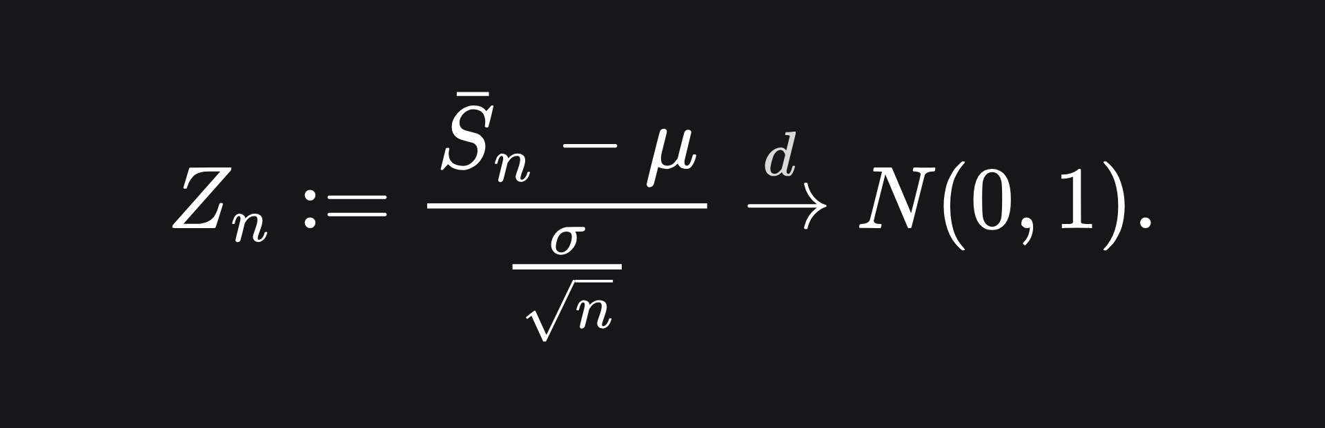
The idea here is that we can transform Z_n back to s̄ by rearranging this formula. Before that, let’s think about properties of the standard Gaussian Z, which Z_n converges to, as we make n larger.

To that end, we can look at the area under the standard Gaussian curve to ascertain, say, a 95% interval in which we believe the value of Z to lie:

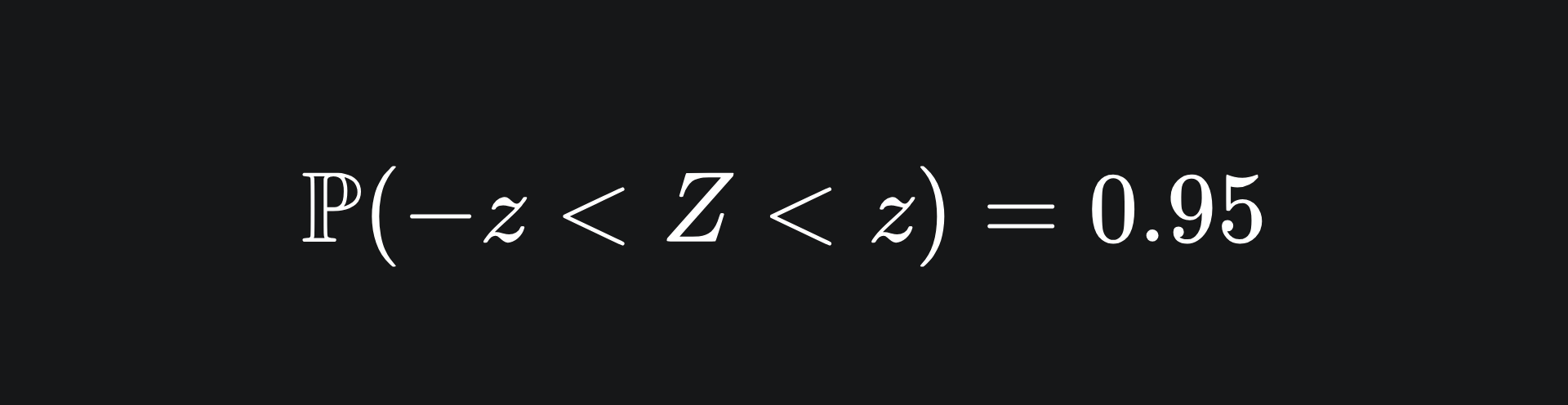
The value that makes this work is z=1.96, but I’ll just leave it as z for now. By the symmetry of the standard Gaussian about z=0, we can represent this visually:

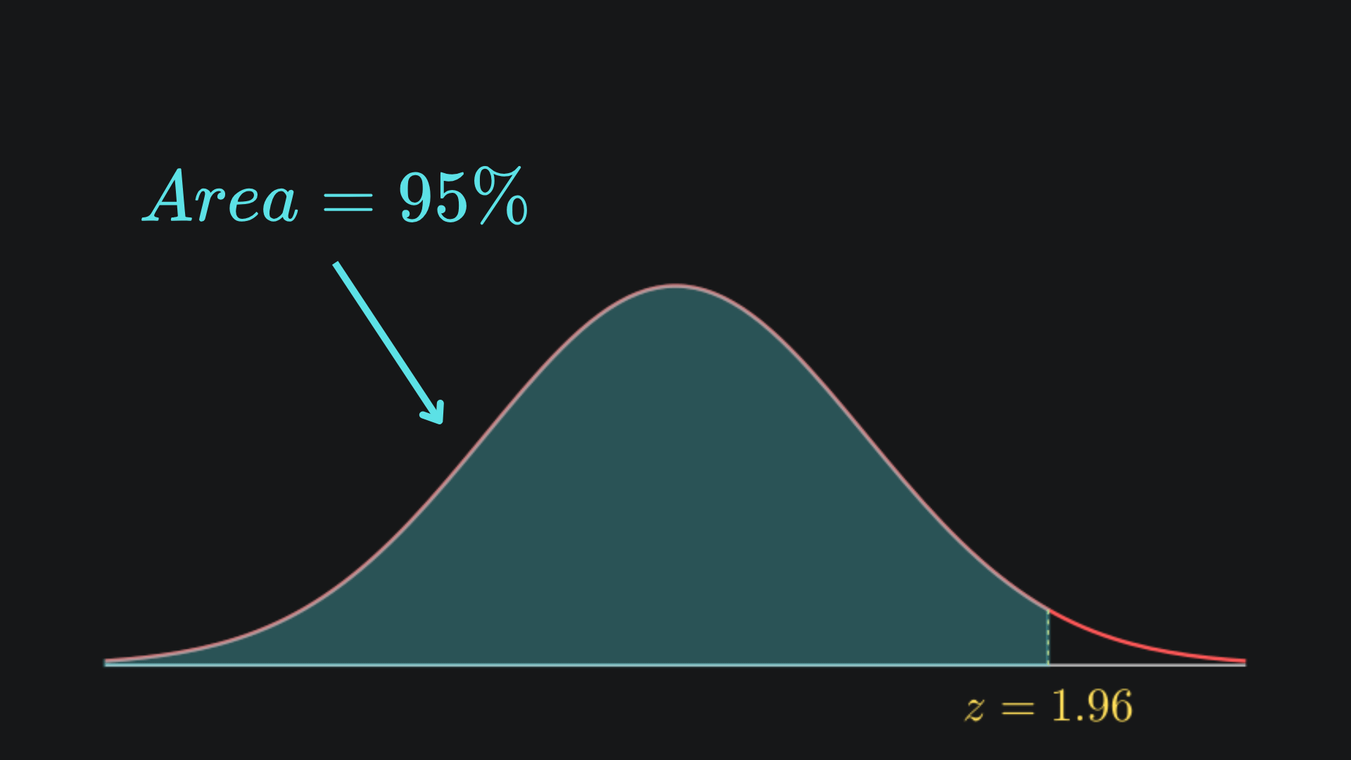
Let’s stick with this 95% example. Substituting the formula for Z_n back in gives

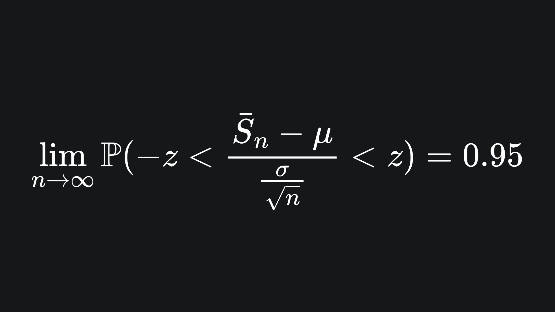
Now, we want to rearrange the inequality to get μ, the value we’ve been looking for this whole time. Check for yourself that this yields the following:

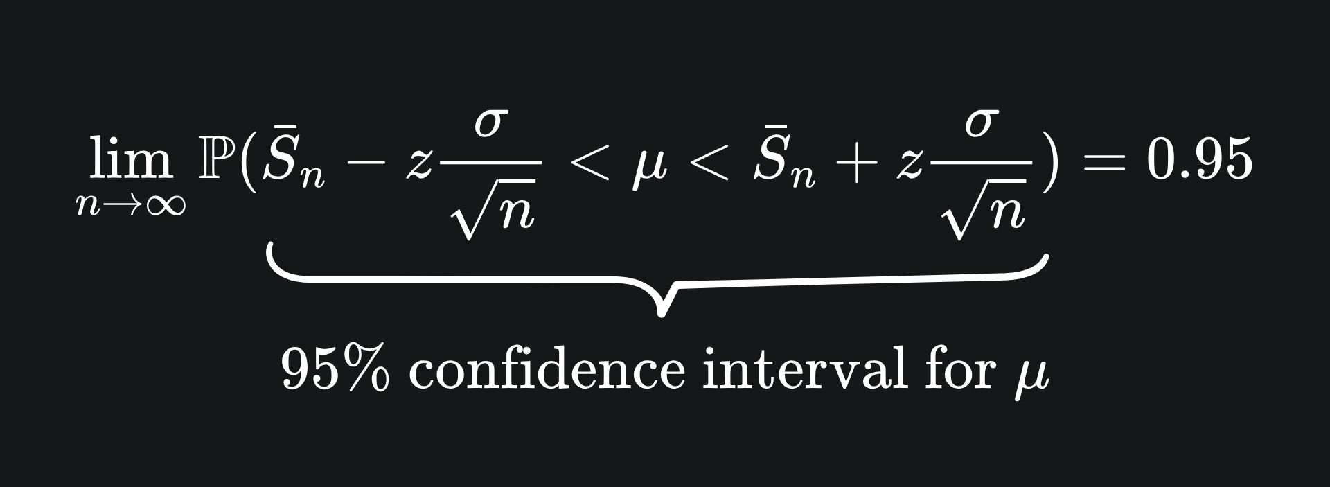
This is a 95% confidence interval for the value of μ. Recall that μ is not a random variable: the sample mean is the probabilistic component.

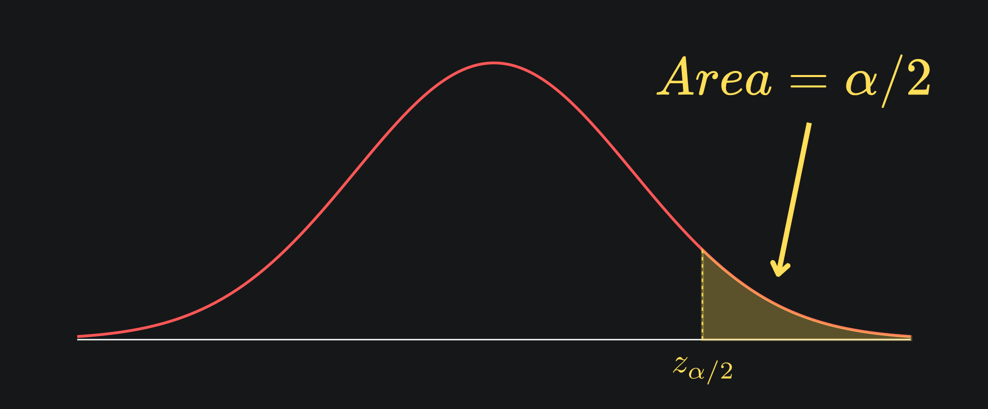
We can generalise this to account for whatever confidence level we want. Let’s define the expression 1-α as our confidence level (this weird-looking formulation would make more sense soon). Let z_α/2 represent the value above which the standard Gaussian has an area under the curve of α/2:

By the symmetry of the standard Gaussian distribution around 0, the area under the curve below -z_α/2 is also α/2:

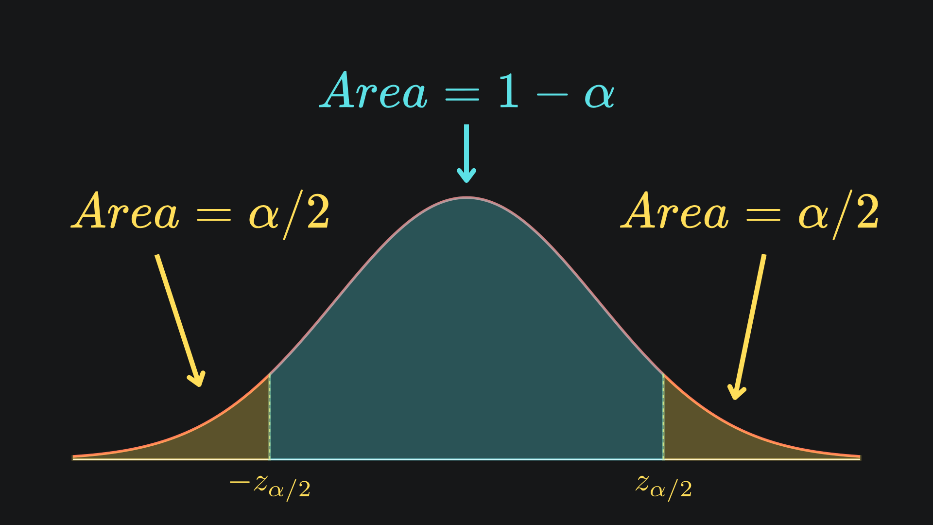
This leaves the area in the middle of (1-α). Mathematically, we have that

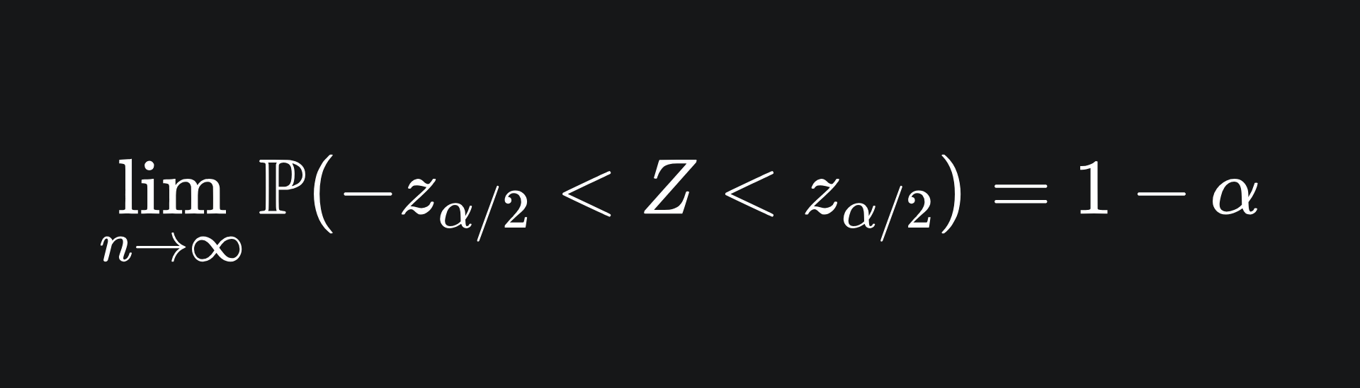
Now, we can rearrange this to isolate the value of μ:

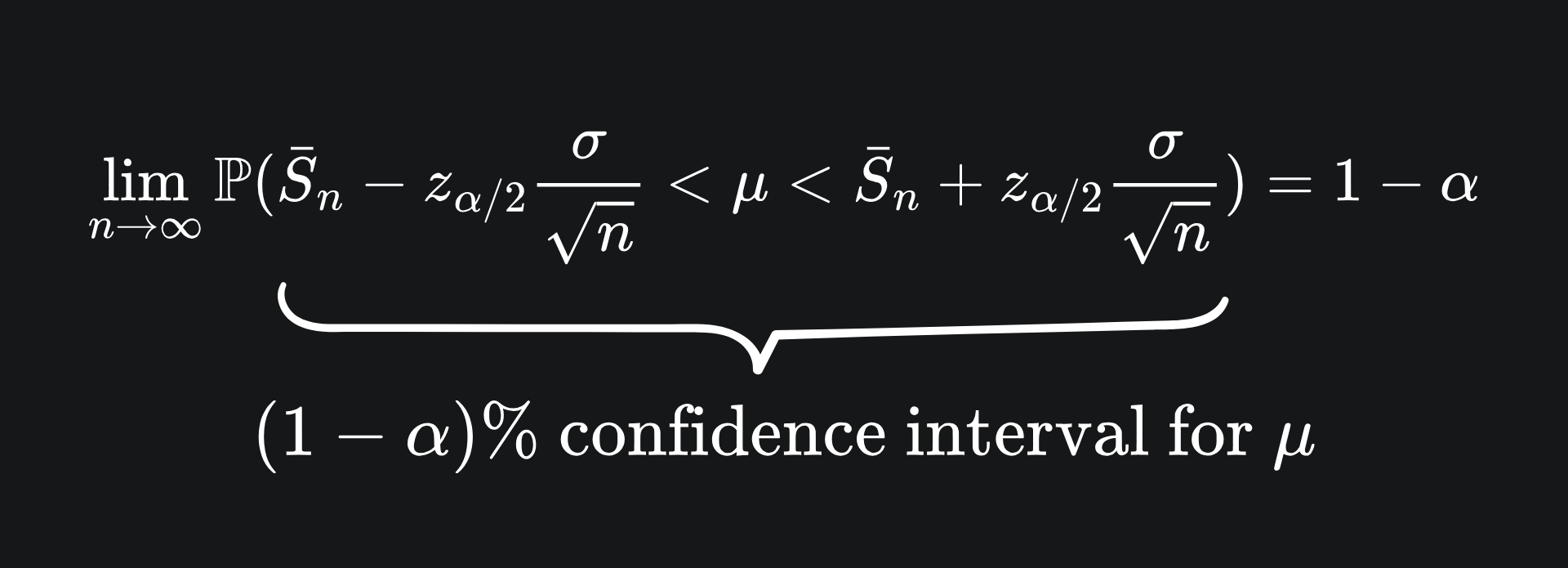
The geometric interpretation hopefully explains why we don’t look for the 100% confidence interval. It’s because the 100% confidence interval captures all possible values from the distribution which, in this case, technically includes all real values. That is to say, a 100% confidence interval for the value of μ includes all real numbers, which doesn’t help us much!

There are two things we can do to make our confidence interval narrower:

💡 Increase the value of α. This constructs a narrower confidence interval but, by definition, we will be less confident that this interval contains the true value of μ.

💡 Increase the value of n. You can hopefully see why this works from the above mathematical derivation thanks to the square root of n in the denonimator. Intuitively though, the more samples we average over, the more likely that it’ll be representative of the true mean μ.²

One more thing: this technique assumes that we know the variance of the distribution. We’ll discuss another time what to do when we don’t know the variance.

What value of n do we need?

The more questions we ask an LLM, i.e. the greater the value of n, the more our sample mean resembles a normal distribution. In turn, this makes our confidence intervals more narrow, i.e. we’re more confident in where we think the true value μ lies.

But this doesn’t actually explain what value of n we need for the result to work. A rule of thumb that I’ve seen online is that a value of n that’s at least 30 is good. That said, I could not find an authentic source to corroborate, so let me know in the comments if you know where that claim comes from. Regardless, the more skewed a distribution is, the larger n is required to achieve a good Gaussian approximation.

Additionally, it is not practical for us to continually prompt an LLM without restraint, due to the token cost associated with invoking the model many times. Thus, the trade-off between additional prompting and eval score confidence must be evaluated on a case-by-case basis.

Packing it all up

We’ve done a lot of heavy lifting in the statistics area today. Next time, we’ll focus more on the LLM eval side, but I figured that this stats lesson would be a good refresher before we get into all that. Plus, who doesn’t love a good Manim snippet?

Here’s the usual roundup:

📦 To estimate the true eval score for an LLM, we would have to prompt the LLM infinitely many times and take the average of the scores. As a compromise, we can instead prompt it a few times, take the average of that sample, and construct a confidence interval that (hopefully) contains the true mean.

📦 The Central Limit Theorem tells us that, under certain conditions, the sample mean converges (in some sense) to a Gaussian distribution. This holds for any probability distribution, continuous or discrete.

📦 The CLT is valuable, because it can be used to help us construct confidence intervals for the true mean, starting with the sample mean.

If you’d like to take your knowledge of the Gaussian to a new dimension (and I mean this quite literally), then check out this article on the Multivariate Gaussian distribution. Slight warning: there’s quite a bit of maths, but there’s also a pretty awesome 3D animation at the end, so definitely worth it.

Training complete!

I hope you enjoyed reading as much as I enjoyed writing 😁

Do leave a comment if you’re unsure about anything, if you think I’ve made a mistake somewhere, or if you have a suggestion for what we should learn about next 😎

Until next Sunday,

Ameer

PS… like what you read? If so, feel free to subscribe so that you’re notified about future newsletter releases:

Sources

• My GitHub repo where you can find the code for the entire newsletter series: link

  • Code for this article: link

• More on the Central Limit Theorem: link to online probability course

• More on convergence in distribution: link to online probability course

1. UK college that is, i.e. 16-18 year old education.

2. This is basically the (weak) Law of Large Numbers.